

Fulton J. Sheen:
The big print giveth, and the fine print taketh away.
Text has been the primary form of documentation in human history. Today large volumes of unstructured text data are being generated and disseminated at an unprecedented pace, via such media as tweets, emails, and scholarly publications. The magnitude of these data has far exceeded our human capacity to read and digest. How can we possibly sift through the world of written text and access what we need? In what ways can computers, which have helped create this ever-growing pile of data, be harnessed to also help us discover relevance and meaning?
Let's start with some basic issues and ideas for processing text.
Imagine having a long legal document, it can be stored digitally along with other documents and files. In its raw text format, you can hardly use the document to compute and compare -- for example, to find other documents related to the same or similar cases -- unless we can convert the text into some numbers to be used in the calculation.
Indeed, the first step of text processing involves a general process called vectorization, which identifies elements in the text and assigns numbers (weights) to them as its numerical representation. The result of this is a list of values, which can then be used for searching, ranking, and association.
Taking single words as basic elements, the following text:
John is quicker than Mary.
can be split into individual tokens John, is, quicker, than, and Mary. In a simple classic approach, we only try to capture what tokens (keywords) occur in the text and pay no heed to the order in which they appear. This is referred to as the bag of words model, which will lead to some loss of information. Apparently, with this treatment, tokenization of the above text will result in the identical bag of words with the following:
Mary is quicker than John.
where the only difference is the order and the meaning is simply the opposite. Indeed, for analyses where the semantic interpretation of a text is critical, the model will suffer from the loss of order. In many practical applications, nonetheless, the bag of words works sufficiently well where the central problem is about finding associations through the keywords. For now, we stick with this basic model and revisit the issue of word order later.
Now that we identify the tokens (words), one may consider normalize them so that the same word types in various forms can be unified and treated as the same.
In English, one can apply normalization techniques such as:
Case folding, which changes all tokens into lower-case, e.g. John and JOHN $\to$ john;
Stemming, which reduces tokens to their roots, e.g. compression and compressed $\to$ compress;
Lemmatization, which converts word variants to their base form, e.g. are and is $\to$ be;
These techniques are language and domain-dependent. Aside from potential benefits of unifying tokens of the same type, token normalization may also lead to undesired consequences, e.g. to treat CAT (the company) and cat as the same. So careful examination of data and application is necessary to determine whether related normalization techniques may be instrumental or detrimental.
Also, note that tokens are not limited to single words. One can use a moving window to take two, three, or more consecutive words at a time to identify all possible phrases or n-grams. Likewise, you can use a moving window to identify any $n$ consecutive characters as tokens. Character n-grams have shown its utility in applications such as spam detection, where junk emails may pad normal keywords with special characters to avoid being identified.
Once tokens -- single words or phrases -- have been identified, they can be sorted and merged into a set of unique tokens, which we refer to as the dictionary. Suppose we have a book collection of The Chronicles of Narnia, for which we only store their titles:
- The Lion, the Witch and the Wardrobe
- The Voyage of the Dawn Treader
- The Horse and His Boy
Based on tokenization of single words with case-folding, the following dictionary (alphabetically ordered) can be identified from this small collection:
| 1 | 2 | 3 | 4 | 5 | 6 | 7 | 8 | 9 | 10 | 11 | |
|---|---|---|---|---|---|---|---|---|---|---|---|
| and | boy | dawn | his | horse | lion | the | treader | voyage | wardrobe | witch |
Now we can use terms in this dictionary to represent each document based on their occurrences, $0$ if one does not occur and $1$ if it does. The following matrix shows such a binary representation:
| 1 | 2 | 3 | 4 | 5 | 6 | 7 | 8 | 9 | 10 | 11 | |
|---|---|---|---|---|---|---|---|---|---|---|---|
| DOC | and | boy | dawn | his | horse | lion | the | treader | voyage | wardrobe | witch |
| 1 | 1 | 0 | 0 | 0 | 0 | 1 | 1 | 0 | 0 | 1 | 1 |
| 2 | 0 | 0 | 1 | 0 | 0 | 1 | 1 | 1 | 1 | 0 | 0 |
| 3 | 1 | 1 | 0 | 1 | 1 | 0 | 1 | 0 | 0 | 0 | 0 |
The size of the dictionary will increase with the size of the text collection and the length of each document. However, one can imagine that, for each document, not all dictionary terms will occur and therefore some (many in fact) of vector values are $0$s. A more efficient representation is a sparse vector, where only non-zero values ($1$ in the binary case here) are retained.
For example, document $3$ in the above matrix can be represented as:
| ( | 1 | 2 | 4 | 5 | 7 | ) |
|---|---|---|---|---|---|---|
| and | boy | his | horse | the |
which only includes terms that appear in the document and have $1$ values.
The binary representation only whether or not a term occurs. This is a reasonable treatment for small text documents such as the above example and tweets.
With longer text documents, when full-text is used for vectorization, it is useful to also consider term frequency (TF).
$TF_{dt}$ is the number of times a term $t$ appears in document $d$.
It is often observed that a term with a higher term frequency in a document is more relevant to the document's topical theme and should, therefore, be given a higher weight.
One can simply use the term frequency as term weight:
$$\begin{aligned} w_{dt} & = & TF_{dt}\end{aligned}$$One can also normalize the TF value with logarithm:
$$\begin{aligned} w_{dt} & = & \begin{cases} 1 + \log TF_{dt}, & \text{if}\ TF_{dt}>0 \\ 0, & \text{otherwise} \end{cases}\end{aligned}$$Example, 3 course titles as documents:
- Information and Systems
- Data and Information
- Systems and System Programming
They can be represented by term frequency (TF):
| Doc# | and | data | information | program | system |
|---|---|---|---|---|---|
| 1. | 1 | 0 | 1 | 0 | 1 |
| 2. | 1 | 1 | 1 | 0 | 0 |
| 3. | 1 | 0 | 0 | 1 | 2 |
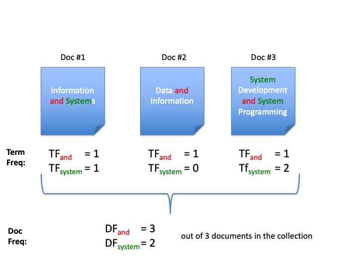
Notice that the term system appears in the 3rd document twice and its term frequency is 2. Other terms either appear in each document once or do not appear at all. So the other values are 0 and 1.
A basic assumption of counting occurrences in the term frequency weight is that all occurrences are equal and should count equally. In light of the Zipf law, however, we know words are used unequally.
Consider a term that appears in many documents/instances such as and
- Stop words: too frequent to be useful
- Frequent terms (used frequently in many documents) are less informative than rare terms
Some words appear more frequently simply because of the effect of least effort. Some are stop-words like a and the that contribute little in meaning. For many of these, there is one thing in common -- they appear frequently not only in the current document but also in other documents as well.
In general, we observe that some terms are used so broadly in so many documents that they can hardly help differentiate one document from another. They are too broad to be specific and informative.
Rare terms:
- More informative than frequent terms
- More specific and better differentiate the document
- We want a high weight for rare terms
On the other extreme, some terms are used in only a very few documents and they very clearly distinguish these documents from others. These terms are rarer, more specific, and should be given more weight according to the observation here.
Imagine we randomly draw a document from the entire text collection, there is a probability that term $t$ will appear, which can be estimated by:
The chance of term $t$ to appear in a document in collection $C$:
$$ p(t) = \frac{n_t}{N} $$- $N$ the total number of documents in the collection
- $n_t$: the number of documents containing term $t$
where $n_t$ is the number of documents containing term $t$ and $N$ is the total number of documents in the collection $C$. $p(t'|C)$ is the complimentary probability that $t$ does NOT occur.
Back to example of 3 course titles:
- Information and Systems
- Data and Information
- Systems and System Programming
Now with the example of three course titles. We can easily computing the probability for each term.
Three documents in the collection: $ N = 3$
| t | $n_t$ | p(t) |
|---|---|---|
| data | 1 | 1/3 |
| program | 1 | 1/3 |
| information | 2 | 2/3 |
| system | 2 | 2/3 |
| and | 3 | 3/3 |
The term data appears in only one document and its probability of appearing is $1/3$. The term and appears in all three documents and its probability is $3/3$ or $100\%$.
For a specific document $d$ where term $t$ appears, it is certain so the probability of observing the term is:
$$\begin{aligned} p(t|d) & = & 1 \\ p(t'|d) & = & 0\end{aligned}$$The amount of information gain or relative entropy, according to chapter [ch:info]{reference-type="ref" reference="ch:info"}, by seeing the term in document $d$ out of collection $C$, can be computed by:
$$\begin{aligned} Info(t) & = & DL[P(t|d) || P(t|C)] \\ & = & - \sum_{x \in (t,t')} p(x|d) \log \frac{p(x|C)}{p(x|d)} \\ & = & - p(t|d) \log \frac{p(t|C)}{p(t|d)} - p(t'|d) \log \frac{p(t'|C)}{p(t'|d)} \\ & = & - 1 \cdot \log \frac{n_t}{N} - 0 \cdot \log \frac{p(t'|C)}{p(t'|d)} \\ & = & - \log \frac{n_t}{N}\end{aligned}$$This information gain of term $t$ is in fact the exactly the classic Inverse Document Frequency (IDF) weighting scheme:
Inverse document frequency (IDF): $$\begin{aligned} IDF_t & = & Info(t) \\ & = & \log \frac{N}{n_t}\end{aligned}$$
where $n_t$, the number of documents with term $t$, is commonly referred to as document frequency (DF).
Again we use the three course titles as an example.
Three documents in the collection: $ N = 3$
| t | $n_t$ | p(t) | $IDF_t$ |
|---|---|---|---|
| data | 1 | 1/3 | $\log{\frac{3}{1}}=0.48$ |
| program | 1 | 1/3 | $\log{\frac{3}{1}}=0.48$ |
| information | 2 | 2/3 | $\log{\frac{3}{2}}=0.18$ |
| system | 2 | 2/3 | $\log{\frac{3}{2}}=0.18$ |
| and | 3 | 3/3 | $\log{\frac{3}{3}}=0$ |
IDF measures how informative a term is when it appears in a document. For a term that appears in all documents in the collection -- the stop-words for example -- $n_t$ is the same as $N$ and its IDF weight becomes:
$$\begin{aligned} IDF_t & = & \log \frac{N}{N} \\ & = & \log 1 \\ & = & 0\end{aligned}$$For a term that appears in very few documents in a large collection, $n_t << N$ and the IDF weight is great. In this way, the IDF weight penalizes broader terms used in many documents and rewards more selective, rare terms.
Please note that IDF is a collection-wide statistic for each term whereas term frequency (TF) is a term statistic specific to a document. They address two separate aspects of term weighting and are often combined for document representation.
The combined weighting scheme, namely the classic $TF\times IDF$, assigns a term's weight by:
$$\begin{aligned} w_{dt} & = & TF_{dt} \times \log \frac{N}{n_t}\end{aligned}$$or with log-transformed TF weight:
$$\begin{aligned} w_{dt} & = & \begin{cases} (1 + \log TF_{dt}) \log \frac{N}{n_t} , & \text{if}\ TF_{dt}>0 \\ 0, & \text{otherwise} \end{cases}\end{aligned}$$where $TF_{dt}$ is the number of times term $t$ occurs in document $d$ (TF), $n_t$ is the number of documents having $t$ (DF), and $N$ is the total number of document in the collection.
Now we can revisit the small collection of three course titles. The TF representation of documents:
TF representation:
| Doc# | and | data | information | program | system |
|---|---|---|---|---|---|
| 1. | 1 | 0 | 1 | 0 | 1 |
| 2. | 1 | 1 | 1 | 0 | 0 |
| 3. | 1 | 0 | 0 | 1 | 2 |
And now that we have the IDF score for each term:
| t | $n_t$ | p(t) | $IDF_t$ |
|---|---|---|---|
| data | 1 | 1/3 | $\log{\frac{3}{1}}=0.48$ |
| program | 1 | 1/3 | $\log{\frac{3}{1}}=0.48$ |
| information | 2 | 2/3 | $\log{\frac{3}{2}}=0.18$ |
| system | 2 | 2/3 | $\log{\frac{3}{2}}=0.18$ |
| and | 3 | 3/3 | $\log{\frac{3}{3}}=0$ |
We can multiple the TF and IDF values for each term in each documents, and we get:
TF*IDF representation:
| Doc# | and | data | information | program | system |
|---|---|---|---|---|---|
| 1. | $$1\times0 = 0$$ | 0 | 0.18 | 0 | 0.18 |
| 2. | 0 | 0.48 | 0.18 | 0 | 0 |
| 3. | 0 | 0 | 0 | 0.18 | $$2\times0.18 = 0.36$$ |
Notice that the term and appears in every document and its TFIDF weight has been reduced to 0. The term system appears in document 3 for 2 times, with a collection wide IDF of 0.18, its TFIDF weight in document 3 is $2\times0.18$, which is 0.36.
In certain applications, TF may be normalized by document length to alleviate potential favoritism toward longer documents.
There are other variations of the TFIDF treatment. This is one of the most widely used term weighting methods in information retrieval and text mining.