
While exploring or modeling data, we often need to look at how variables may be related to one another, what data instances may share similarities, and what major clusters or themes may exist in the data. The common task here is to measure the similarity, proximity or distance between two entities, such as two variables or two data instances.
Many related similarity and distance measures are based on the concepts of sets and vectors. So let's review them before we look at similarities and distances.
A set is
a collection of member objects or elements.
- Elements: unique entities, symbols, names, and/or numbers
- Cardinality: # elements
We have discussed categorical variables with values from a set of labels. A set is a collection of member objects or elements. The elements can be any unique entities, symbols, names, and/or numbers. The number of elements in a set is referred to as its {\it cardinality}.
A tweet, for example, can be treated as a set of words appearing in it. In this case, the elements are the words and the cardinality is the number of unique words in the tweet.
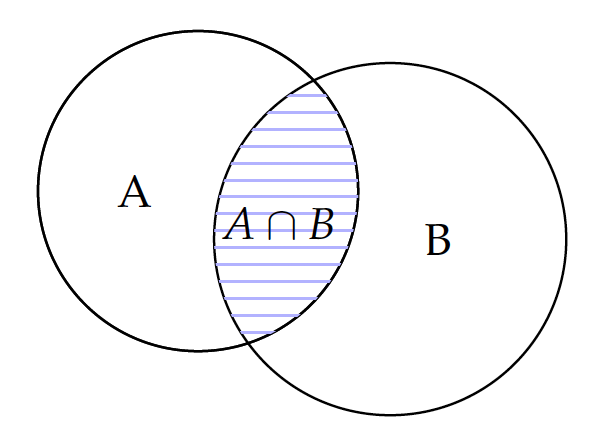
Consider the skill sets of two data science teams A and B.
It is easy to count the number of skills in each team and identify their cardinalities: $|A|=4$ and $|B|=5$.
Their intersection or what they have in common is the set containing math and SQL, which is illustrated by the shaded area in the figure. The interaction operation is communicative, i.e. $A \cap B=B \cap A$, because the order does not matter.
Union
A = {AI, Math, Python, SQL}
B = {InfoVis, Math, R, SQL, Stats}
Union $\cup$ (OR)
\begin{eqnarray*} A \cup B & = & \{AI, InfoVis, Math, Python, R, SQL, Stats\} \end{eqnarray*}\begin{eqnarray*} |A \cup B| & = & |A| + |B| - |A \cap B| \\ & = & 4 + 5 - 2 \\ & = & 7 \end{eqnarray*}what are all the elements?
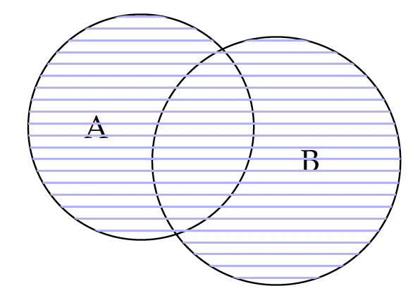
Now, if we are to put the two teams together on one project, the overall skill set of the merged project team will be the union of the two. Because a set contains only unique elements, those in the intersection $A \cap B$ will have duplicates when two sets are combined and should be removed by subtracting the intersection $|A \cap B|$.
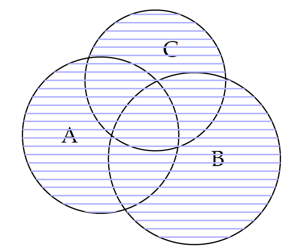
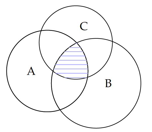
The union operation is also communicative, i.e. $A \cup B = B \cup A$, because it does not matter whether we add B to A or A to B. In addition, both the union and intersection operations have the associative property, that is:
\begin{eqnarray*} (A \cup B) \cup C & = & A \cup (B \cup C) \\ (A \cap B) \cap C & = & A \cap (B \cap C) \end{eqnarray*}for any sets A, B, and C. As illustrated in figure 1, we will obtain the same union set (the shaded circles) regardless of which two are combined first. The same is true with intersection, as illustrated in figure 2.
The union ($\cup$) operation is similar to {\it addition} ($+$), whereas the intersection {$\cap$} operation can be likened to {\it multiplication} ($\times$). For demonstration, let's look at a couple of special cases. Let $0$ denote an empty set, with no elements at all; $1$ be the the universal set, containing all elements in the universe.
For a regular set $A$, we can show the similarity between union ($\cup$) and addition ($+$).
The union of a set A and an empty set $0$ is the A itself: $A \cup 0=A$. The same is true about adding an empty set $0$ to the universal set $1$. $1 \cup A$ is not exactly $1 + A$, but they are roughly the same as long as the universal set $1$ is far greater than A.
Likewise, intersection ($\cap$) and multiplication ($\times$) operations are similar.
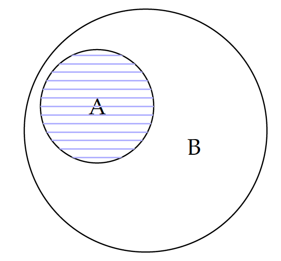
The intersection between any set (A or 1) and an empty set 0 is always an empty set: $A \cap 0 = 0$ and $1 \cap 0=0$. The intersection between a set A and the universal set $1$ is A, because the universal includes A as a subset. In fact, for any set A that is a subset of B, their intersection is A and their union is B:
\begin{eqnarray} A \cap B & \stackrel{\forall A \in B}{=} & A \\ A \cup B & \stackrel{\forall A \in B}{=} & B \end{eqnarray}Now we have looked at the similarities of intersection vs. multiplication, and union vs. addition. The notion of set is applicable to events in probabilities. In fact, the notion of intersection is applicable to the joint probability of multiple events, which can be computed by multiplication. Union, on the other hand, is related to the OR probability, for which probabilities are added toghether.
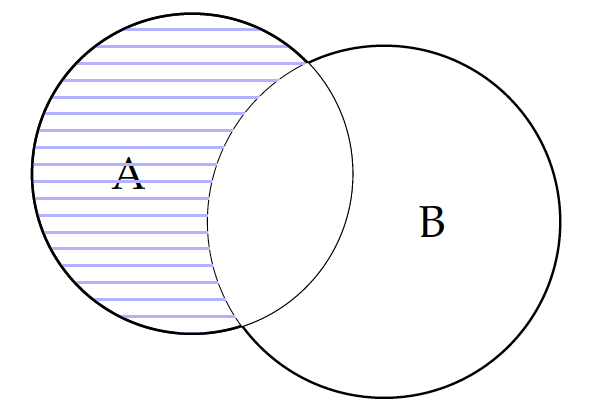
Besides union and intersection operators that can be likened to addition and multiplication, there is also the subtraction operator on sets. For two sets $A$ and $B$, $A-B$ computes the difference between A and B, or the elements of A that do not appear in B. This is essentially the removal of their intersection from set A, as shown in the figure.
The cardinality of the subtracted set can be computed by $|A| - |A \cap B|$.
If A and B have no intersection, $A-B$ is the same as A. If A is a subset of B, then the result is an empty set. Subtraction is not communicative, as $A-B \ne B-A$.
A vector is:
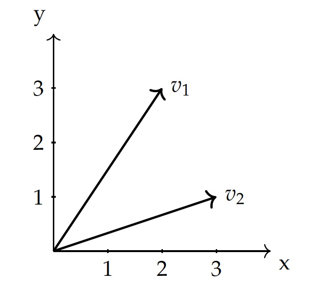
\begin{eqnarray*} v_1 & = & (2,3) \\ v_2 & = & (3,1) \end{eqnarray*}an entity having both a magnitude and a direction
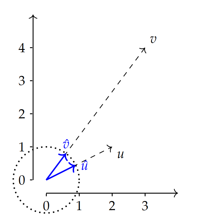
In geometrical terms, a {\it vector} is an entity having both a magnitude (length) and a direction, in a vector space with multiple dimensions.
The figure shows data $v_1$ and $v_2$ in a space with $X$ and $Y$ dimensions. In the vector space, each data point is a vector from the origin $(0,0)$, as shown as directed lines in the figure, and can be represented by its dimensional values.
So in this representation, a vector is simply a list of its coordinate values, each of which represents a feature dimension (variable). The greater the number of dimensions, the longer the list of the values.
A {\it set} can be represented as a vector. For example, suppose $\{$AI, InfoVis, Math, Python, R, SQL, Stats$\}$ is a comprehensive set of skills for data science teams. Given the A and B teams and their skills we discussed earlier, we can have the binary representation show in the table, where $0$ represents the absence of a skill and $1$ denotes the presence of the skill.
By populating the 0 and 1 values in a fixed order of the skills, we obtain the vector representations for teams A and B identical to the table. The vector space has $7$ dimensions, which correspond to seven skills in the comprehensive set, to represent instances of data science teams. These vectors are {\it row vectors} as they represent data instances.
Note we use superscripted $A^T$ and $B^T$, where $T$ is the {\it transpose} operator, because of the convention of using column vectors by default.
By transposing the column vectors A and B -- with a $90^\circ$ counterclockwise rotation -- we obtain the row vectors $A^T$ and $B^T$:
Here, each column vector is a column with $7$ rows of {\it real} numbers. Hence, $A \in \R^m$ and $B \in \R^m$, where $m=7$. By transposing the column vectors, we obtain row vectors, each of which has $m=7$ columns of {\it real} numbers.
With the ideas of sets and vectors, it is now easier to discuss several classic similarity or distance measures.
- How similar or related two data instances are?
- Simiarity, dissimilarity, proximity, distance...
- Lower and upper limits vary
Let's first look at similarities based on sets, the Dice and Jaccard coefficients.
Dice coefficient of sets A and B is 2 times the cardinality of A, B intersection divided by the sum of their cardinalities.
Jaccard's coefficient is similar: the cardinality of AB intersection divided by the cardinality of their union.
Example to compute Dice:
A = {AI, Math, Python, SQL}
B = {InfoVis, Math, R, SQL, Stats}
- $| A \cap B | = | \{Math, SQL\} | = 2$
First, compute the cardinality of the intersection.
- $| A | = 4$, $| B | = 5$
And compute the cardinalities of A and B.
The Dice coefficient becomes:
$Dice(A,B) = \frac{2 |A \cap B|}{|A| + |B|} = \frac{2 \times 2}{4 + 5} = \frac{4}{9}$
Example to compute Jaccard:
A = {AI, Math, Python, SQL}
B = {InfoVis, Math, R, SQL, Stats}
- $| A \cap B | = | \{Math, SQL\} | = 2$
Again, compute the cardinality of intersection.
- $| A \cup B | = | \{AI, InfoVis, Math, Python, R, SQL, Stats\} | = 7$
And the cardinality of the union.
Jaccard is the ratio of the intersection to the union:
$Jaccard(A,B)= \frac{|A \cap B|}{|A \cup B|} = \frac{2}{7}$
When $P=1$, $L^1$ is Manhattan distance: $\sum_i |u_i - v_i|$, sum of absolute distances along the dimensions.
When $P=2$, $L^2$ is the Euclidean distance: $\sqrt{\sum_i |u_i - v_i|^2}$, the line distance of two points.
Example vectors:
| Team | AI | InfoVis | Math | Python | R | SQL | Stats |
|---|---|---|---|---|---|---|---|
| U | 1 | 0 | 1 | 1 | 0 | 1 | 0 |
| V | 0 | 1 | 1 | 0 | 1 | 1 | 1 |
$L^1$, Manhattan distance: \begin{eqnarray} D(U,V) & = & |1-0| + |0-1| + |1-1| + |1-0| + |0-1| + |1-1| + |0-1| \\ & = & 1+1+0+1+1+0+1 \\ & = & 5 \end{eqnarray}
For $L^1$ norm, which is Manhattan distance, we compute the difference for each dimension, i.e. each column here, and get the sum of their absolute values.
$L^2$, Euclidean distance: \begin{eqnarray} D(U,V) & = & \sqrt{|1-0|^2 + |0-1|^2 + |1-1|^2 + |1-0|^2 + |0-1|^2 + |1-1|^2 + |0-1|^2} \\ & = & \sqrt{1+1+0+1+1+0+1} \\ & = & \sqrt{5} \end{eqnarray}
For L2 norm, which is Euclidean distance, the difference here is that we need to compute the square of the subtraction, add them up, and then take the square root of the sum.
Here, the Euclidean distance happens to be the square root of the Manhattan distance because of the binary representation. This is only a special case and you will see that they behave very differently with real numbers.
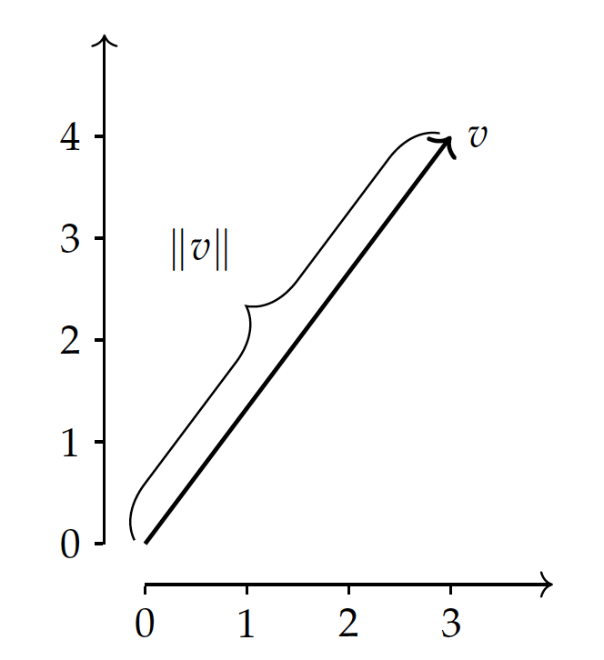
The magnitude or length of a vector is in fact the Euclidean distance from the origin. So this can be considered as an application of the Minkowski distance of $L^2$ norm.
The dot product of two vectors is to multiply values of the two on each dimension and take the sum. This is the covariance of values in the two vectors and the final score is impacted by three factors: the vector magnitudes of $u$ and $v$, and the alignment of the two vectors, or to what degree they point to the same direction.
In particular, you can think of the dot product as the product of 1) the degree pointing to the same direction, times 2) u magnitude, times 3) v magnitude.
Now that we know the dot product is the product of the three factors, if we normalize or divide it by the product of the two vector magnitudes, the result is reduced to their direction similarity, or to be precise, the Cosine similarity.
Example vectors:
| Team | AI | InfoVis | Math | Python | R | SQL | Stats |
|---|---|---|---|---|---|---|---|
| U | 1 | 0 | 1 | 1 | 0 | 1 | 0 |
| V | 0 | 1 | 1 | 0 | 1 | 1 | 1 |
Let's revisit the example vectors and see how we can compute their Cosine similarity.
- Dot product: $u \cdot v = \sum_i u_i v_i = 1\times0 + 0\times1 + .. + 0\times1 = 2$
First, we compute their dot product to find out how much the covary.
- $u$ magnitude: $||u|| = \sqrt{\sum_i u_i^2} = \sqrt{1^2 + 0^2 + 1^2 + 1^2 + 0^2 + 1^2 + 0^2} = \sqrt{4} = 2$
Then, we compute the magnitudes of u and v.
- $v$ magnitude: $||u|| = \sqrt{\sum_i v_i^2} = \sqrt{0^2 + 1^2 + 1^2 + 0^2 + 1^2 + 1^2 + 1^2} = \sqrt{5}$
Finally:
\begin{eqnarray} Cosine(u, v) & = & \frac{u \cdot v}{||u|| \times ||v||} \\ & = & \frac{2}{2\times\sqrt{5}} \end{eqnarray}The Cosine similarity measures the Cosine of the angle between two vectors. It is all about the direction and the magnitude of each vector does not matter -- you see in the cosine formula, it has been normalized by those magnitudes. Cosine varies from -1 to 1. Cosine reaches its maximum $1$ when two vectors point to the exact same direction; its minimum $-1$ when the two vectors point to the opposite direction; Cosine is $0$ when the vectors are orthogonal or perpendicular to each other.
Cosine similarity is particularly useful in applications where the distribution of values is more important rather than absolute values. For example, in text mining, it is more important to find out frequencies of terms relative to one another. Cosine similarity has performed very well in these applications.