Search
Python Data Preprocessing

Data Quality

  • Today’s real-world data likely origins from multiple, heterogeneous sources
  • Therefore, we are very likely to handle low-quality data
  • It is important to properly address data quality issues
  • Even simple descriptive analysis can be applied such that:
    • Sort all values in ascending or descending order
      1. If all values are identical: no information. Ignore this variable!
      2. If some values occur abnormally with very high frequency (e.g., "Alabama" in 20% cases for state entry: need to examine whether it is caused by any interesting pattern (e.g., football fan survey) or error (e.g., default value)
  • All techniques (e.g., data cleaning, integration, reduction, transformation, and discretization) related to data quality need to be properly addressed

In this exercise, we are going to utilize a dataset distributed as a part of the Yelp Dataset Challenge (https://www.yelp.com/dataset). The ultimate goal is to create a classifier to predict the usefulness of each review by using various attributes. For instance, the count of words can be a good indicator of the usefulness of reviews because longer reviews can deliver more information than shorter reviews can do. The sentiment of reviews might be important because too positive/negative reviews might not be objective. Metrics related to social networks such as degree, betweenness, and eigenvector might be important by representing the social status of reviewers. To achieve the ultimate goal, preprocessing data is the first step. Let's open the data. There are 1,000 tuples and 26 attributes. The names of attributes are self-explanatory.

## Imports all necessary modules
import pandas as pd
import matplotlib.pyplot as plt
import numpy as np
import seaborn as sns
from numpy import linalg
from scipy import stats

## This loads the csv file from disk
yelp_data = pd.read_csv(
    filepath_or_buffer = "./data/Yelp_Usefulness_Practice.csv", sep = ",", header=0 )

print(yelp_data.head(20))
## print the dimension of the data
print(yelp_data.shape)
                   review_id  review_stars  word_count  lexical_diversity  \
0     bRGHgwAd3zfiiDMT9JyKcA             1          23           0.869565   
1     TK-0pfhHorvwZK0YhDe2fQ             5          26           0.769231   
2     XTOQ6blQzzzoK26QRJl3zg             5          71           0.760563   
3     KA9VwKYL-7I2LuQnXeuEBw             5          74           0.689189   
4     C2kblEfR4oMWR9oGhYN2cQ             5          31           0.903226   
5     mTA_VwPiWw6cubKHAsrIkQ             5          32           0.875000   
6     cnZI2W7C-D_w38WHMRer3w             1         124           0.572581   
7     UlxgrLCL9WOjJL5hZ1Zd9A             2         374           0.631016   
8     P5Sx85NU3sALCtbOx1Qgvg             2          45           0.888889   
9     Agb8ItmoRPyXPdQ8jLEgJw             4          60           0.633333   
10    g-JmmzYa4PDRKTWhuXPurg             5          21           0.761905   
11  "-jxAByrXxlQXMYbx-s37JQ"             5          97           0.762887   
12    pvfpk0afGKhCm_6eHF2HUg             4          16           0.812500   
13    64awIJhFkvTsi7HVgYYkpg             4         212           0.589623   
14    2-u_hm8jJmT6NmE2CXmEvw             4          20           0.850000   
15    p9I2_QDn8FXRDlZmsYRe-w             1          37           0.783784   
16    ERv4db1Jd0qUkC0puEIwNg             5          42           0.785714   
17    _GKA5Jp1kxxYkvJT1yTysw             1          45           0.822222   
18    Kd0fUE3pHbouy5PANkisxQ             4         170           0.658824   
19    b_XQ2S7qomhBtqTEi3EKIQ             2          81           0.802469   

    correct_spell_ratio  price_included  procon_included  joy      love  \
0              0.869565        0.000000                0  0.0  0.000000   
1              0.846154        0.000000                0  0.0  0.000000   
2              0.943662        0.014085                0  0.0  0.000000   
3              0.905405        0.000000                0  0.0  0.000000   
4              0.903226        0.000000                0  0.0  0.000000   
5              0.812500        0.031250                0  0.0  0.000000   
6              0.959677        0.008065                0  0.0  0.000000   
7              0.882353        0.000000                0  0.0  0.002667   
8              0.777778        0.000000                0  0.0  0.000000   
9              0.883333        0.000000                0  0.0  0.000000   
10             0.952381        0.000000                0  0.0  0.000000   
11             0.804124        0.010309                0  0.0  0.000000   
12             1.000000        0.000000                0  0.0  0.000000   
13             0.900943        0.000000                0  0.0  0.000000   
14             0.950000        0.000000                0  0.0  0.000000   
15             0.810811        0.000000                0  0.0  0.000000   
16             0.880952        0.023810                0  0.0  0.000000   
17             0.911111        0.000000                0  0.0  0.000000   
18             0.835294        0.011765                0  0.0  0.000000   
19             0.901235        0.037037                0  0.0  0.000000   

    affection  ...  distress  FleschReadingEase  user_review_count  \
0         0.0  ...       0.0            81.1310                  5   
1         0.0  ...       0.0            48.9568                 22   
2         0.0  ...       0.0            95.9393                 10   
3         0.0  ...       0.0            86.9222                  1   
4         0.0  ...       0.0            63.0018                 19   
5         0.0  ...       0.0            83.5138                192   
6         0.0  ...       0.0            79.5758                  3   
7         0.0  ...       0.0            70.6751                459   
8         0.0  ...       0.0            91.7543                 45   
9         0.0  ...       0.0            77.6478                  3   
10        0.0  ...       0.0            74.0150                246   
11        0.0  ...       0.0            63.5937                265   
12        0.0  ...       0.0            63.4338                 28   
13        0.0  ...       0.0            79.9034                 10   
14        0.0  ...       0.0           106.7450                  4   
15        0.0  ...       0.0            63.1022                 40   
16        0.0  ...       0.0            89.8948                 44   
17        0.0  ...       0.0            76.9711                  2   
18        0.0  ...       0.0            68.1763               1261   
19        0.0  ...       0.0            83.4026                  3   

    yelping_months  degree  betweenness  eigenvector  business_stars  \
0               24       0     0.000000     0.000000             3.0   
1                6       1     0.000000     0.000000             4.5   
2               14       0     0.000000     0.000000             4.5   
3                3       0     0.000000     0.000000             5.0   
4               40       0     0.000000     0.000000             3.5   
5               34      16     0.000035     0.006457             5.0   
6                8       1     0.000000     0.000004             4.5   
7               58      51     0.000007     0.024421             4.0   
8               74       0     0.000000     0.000000             5.0   
9                3       0     0.000000     0.000000             4.5   
10              80       1     0.000000     0.000000             4.0   
11              74      32     0.000133     0.017016             4.5   
12              15       0     0.000000     0.000000             2.5   
13               3       0     0.000000     0.000000             4.0   
14               5       4     0.000010     0.000377             3.0   
15              25       2     0.000001     0.000418             3.5   
16              81      12     0.000107     0.001598             4.0   
17              17       0     0.000000     0.000000             2.5   
18              76      12     0.000088     0.001898             3.5   
19               8       0     0.000000     0.000000             4.0   

    business_review_count       class  
0                      40      useful  
1                     319      useful  
2                     535  not_useful  
3                      28      useful  
4                      84      useful  
5                      19      useful  
6                     692      useful  
7                      47      useful  
8                     290      useful  
9                      20  not_useful  
10                    122  not_useful  
11                    168      useful  
12                     30  not_useful  
13                    446  not_useful  
14                    136  not_useful  
15                     31      useful  
16                    569      useful  
17                    123      useful  
18                   4967      useful  
19                     60  not_useful  

[20 rows x 26 columns]
(1000, 26)

Applying descriptive analysis

As explained earlier, we can apply a descriptive analysis to understand the distribution of data. We can count the number of unique values as well.

## Set the maximum number of columns as "None" to display all columns
pd.set_option('display.max_columns', None)

## Pandas' describe method can provide basic statistics for numeric variables at default
print(yelp_data.describe())
       review_stars   word_count  lexical_diversity  correct_spell_ratio  \
count   1000.000000  1000.000000        1000.000000          1000.000000   
mean       3.604000    87.588000           0.770577             0.881534   
std        1.534124    85.127098           0.100830             0.055464   
min        1.000000     3.000000           0.438134             0.444444   
25%        2.000000    32.000000           0.703216             0.850000   
50%        4.000000    58.000000           0.771373             0.886020   
75%        5.000000   112.000000           0.838710             0.914679   
max        5.000000   664.000000           1.000000             1.000000   

       price_included  procon_included          joy         love    affection  \
count     1000.000000      1000.000000  1000.000000  1000.000000  1000.000000   
mean         0.006003         0.003000     0.000016     0.002612     0.000011   
std          0.012553         0.054717     0.000502     0.009139     0.000238   
min          0.000000         0.000000     0.000000     0.000000     0.000000   
25%          0.000000         0.000000     0.000000     0.000000     0.000000   
50%          0.000000         0.000000     0.000000     0.000000     0.000000   
75%          0.006993         0.000000     0.000000     0.000000     0.000000   
max          0.100000         1.000000     0.015873     0.105263     0.005848   

           liking   enthusiasm      sadness  dislike      despair  \
count  997.000000  1000.000000  1000.000000   1000.0  1000.000000   
mean     0.000002     0.000024     0.000068      0.0     0.000022   
std      0.000055     0.000358     0.000980      0.0     0.000703   
min      0.000000     0.000000     0.000000      0.0     0.000000   
25%      0.000000     0.000000     0.000000      0.0     0.000000   
50%      0.000000     0.000000     0.000000      0.0     0.000000   
75%      0.000000     0.000000     0.000000      0.0     0.000000   
max      0.001724     0.007463     0.022727      0.0     0.022222   

            horror     distress  FleschReadingEase  user_review_count  \
count  1000.000000  1000.000000        1000.000000        1000.000000   
mean      0.000642     0.000071          78.880178         123.636000   
std       0.004129     0.000721          13.644488         331.058843   
min       0.000000     0.000000         -37.145400           1.000000   
25%       0.000000     0.000000          72.448250           6.000000   
50%       0.000000     0.000000          80.073150          21.000000   
75%       0.000000     0.000000          86.875000          96.000000   
max       0.058824     0.011111         118.175000        3448.000000   

       yelping_months       degree  betweenness  eigenvector  business_stars  \
count     1000.000000  1000.000000  1000.000000  1000.000000      1000.00000   
mean        33.541000    21.222000     0.000397     0.005586         3.78800   
std         23.902252    65.381874     0.002117     0.017273         0.74774   
min          1.000000     0.000000     0.000000     0.000000         1.00000   
25%         13.000000     0.000000     0.000000     0.000000         3.50000   
50%         30.000000     1.000000     0.000000     0.000000         4.00000   
75%         51.000000     8.000000     0.000087     0.001192         4.50000   
max        114.000000   722.000000     0.038897     0.140342         5.00000   

       business_review_count  
count            1000.000000  
mean              379.584000  
std               652.676672  
min                 3.000000  
25%                42.000000  
50%               150.000000  
75%               416.750000  
max              6200.000000  
## In the above, only 24 attributes got results.
## We need to select "only" categorical attributes to get descriptive statistics for categorical attributes
print(yelp_data[["review_id", "class"]].describe())
                     review_id       class
count                     1000        1000
unique                    1000           2
top     dw7JgmhbFL_VDRqYzZ4nVA  not_useful
freq                         1         507

For the categorical attributes, we found that there are no cases such that all values are identical or some values occur abnormally with very high frequency.

However, in the case of numeric attributes, we found that there are three missing values in the "liking" attribute. The total count of tuples is 997, although all other attributes' count is 1,000. We can also check missing values by using Pandas' isna method. Also, "dislike" attribute has all zero values. That said, we need to drop this attribute by using Pandas' drop method. However, we will keep this for now.

## Show the number of data per attributes that has missing values
print(yelp_data.isna().sum())
review_id                0
review_stars             0
word_count               0
lexical_diversity        0
correct_spell_ratio      0
price_included           0
procon_included          0
joy                      0
love                     0
affection                0
liking                   3
enthusiasm               0
sadness                  0
dislike                  0
despair                  0
horror                   0
distress                 0
FleschReadingEase        0
user_review_count        0
yelping_months           0
degree                   0
betweenness              0
eigenvector              0
business_stars           0
business_review_count    0
class                    0
dtype: int64
## check the missing values across tuples of the "liking" attribute
print(yelp_data["liking"].isna())
0      False
1      False
2      False
3      False
4      False
       ...  
995    False
996    False
997    False
998    False
999    False
Name: liking, Length: 1000, dtype: bool

Now, let's create a box plot to see the distribution of the "liking" attribute. This will help us to determine how to handle the missing data.

## Initialize a 6 x 6in figure
fig = plt.figure(figsize = (6, 6))

## Make the box plot
plt.boxplot(
    ## We beed to drop tuples that include missing values
    yelp_data["liking"][~yelp_data["liking"].isna()], labels = ["Liking"]
)

## Adjust the tick and label font size
plt.tick_params(labelsize = 15)

## Set the title
plt.title("The normalized number of words related to 'liking' sentiment", fontsize = 15)
Text(0.5, 1.0, "The normalized number of words related to 'liking' sentiment")

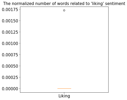
It seems that most of the values are zeros except for one tuple. It is skewed. Therefore, it might be better to use the median central tendency.

## We should exclude missing tuples to get median
median = np.median(yelp_data["liking"][~yelp_data["liking"].isna()])
print ("The median is: ", median)

## Replace missing values with median 
yelp_data["liking"].fillna(median, inplace=True)

## Check whether the missing value were filled
print(yelp_data.isna().sum())
The median is:  0.0
review_id                0
review_stars             0
word_count               0
lexical_diversity        0
correct_spell_ratio      0
price_included           0
procon_included          0
joy                      0
love                     0
affection                0
liking                   0
enthusiasm               0
sadness                  0
dislike                  0
despair                  0
horror                   0
distress                 0
FleschReadingEase        0
user_review_count        0
yelping_months           0
degree                   0
betweenness              0
eigenvector              0
business_stars           0
business_review_count    0
class                    0
dtype: int64

Outlier Detection

We can use Z-score and IQR score to detect ourliers. There are other methods, too.

## The first attribute (review_id) and the last attribute (class) are categorical
## Therefore, we cannot calculate z-score 
## The "dislike" attribute has 0 mean and sd. Therefore, we cannot calculate z score.
## We create indices that exclude review_id, dislike, and class
positions = list(range(1,13))
positions.extend(list(range(14,25)))

z = np.abs(stats.zscore(yelp_data.iloc[:, positions]))
print(z)
[[1.69823455 0.75910397 0.98222214 ... 0.32357593 1.05436955 0.52055472]
 [0.91042067 0.72384491 0.01336026 ... 0.32357593 0.95267909 0.09287036]
 [0.91042067 0.19495907 0.09936362 ... 0.32357593 0.95267909 0.23824012]
 ...
 [0.91042067 0.00691077 0.57485348 ... 0.32357593 0.95267909 0.52821931]
 [0.25825687 0.46320997 0.45810599 ... 0.32357593 1.72338577 0.55427893]
 [1.04607074 2.76680163 2.54659861 ... 0.32357593 1.72338577 0.53128515]]

The above numbers represent z scores of our data. It is difficult to say which data point is an outlier. Let’s try and define a threshold to identify an outlier. To be conservative, we will use 3 as a threshold. We can exclude 0.3% of data.

threshold = 3
print(np.where(z > 3))
(array([  7,  18,  18,  20,  21,  32,  38,  42,  44,  44,  52,  64,  64,
        69,  69,  69,  69,  69,  69,  72,  76,  76,  77,  78,  79,  82,
        82,  89, 102, 106, 121, 121, 124, 129, 135, 146, 150, 151, 152,
       152, 152, 160, 162, 168, 178, 179, 186, 193, 195, 200, 205, 211,
       212, 212, 212, 221, 225, 226, 226, 228, 232, 238, 242, 243, 262,
       262, 262, 262, 262, 262, 263, 267, 277, 281, 286, 291, 291, 299,
       301, 312, 321, 323, 323, 323, 328, 330, 332, 332, 335, 336, 338,
       338, 340, 341, 348, 349, 350, 353, 360, 373, 373, 373, 373, 373,
       374, 375, 375, 375, 379, 385, 385, 385, 386, 394, 395, 406, 406,
       406, 406, 412, 423, 424, 425, 432, 436, 437, 437, 442, 442, 442,
       449, 452, 454, 455, 456, 466, 474, 478, 478, 483, 484, 486, 491,
       493, 497, 503, 505, 507, 511, 512, 512, 512, 516, 519, 520, 520,
       520, 521, 522, 523, 534, 540, 543, 547, 552, 555, 561, 563, 563,
       565, 566, 580, 582, 585, 585, 585, 585, 585, 588, 594, 597, 602,
       615, 628, 635, 638, 638, 638, 638, 639, 644, 646, 647, 650, 660,
       663, 664, 664, 668, 671, 676, 687, 687, 687, 692, 692, 692, 692,
       695, 695, 700, 704, 717, 736, 752, 753, 756, 762, 762, 770, 778,
       778, 778, 784, 785, 791, 794, 802, 805, 807, 814, 821, 823, 823,
       823, 826, 831, 837, 840, 843, 854, 855, 856, 861, 878, 890, 891,
       895, 901, 901, 901, 909, 910, 910, 910, 915, 922, 928, 929, 930,
       930, 944, 945, 950, 957, 964, 969, 974, 974, 974, 992, 994, 998]), array([ 1, 16, 22,  5, 22, 14,  4,  7, 18, 20, 13,  1,  2,  1, 15, 16, 18,
       19, 20,  7,  1, 21,  7,  7,  3,  4, 15, 13, 14,  4,  3,  7,  7,  4,
        7,  4,  3, 11, 14, 18, 19,  7, 22,  7, 15,  3, 14, 11, 13,  4,  7,
       13, 16, 18, 20,  1,  1, 18, 20, 18, 13,  4, 22,  7,  1, 15, 16, 18,
       19, 20, 21, 22,  7,  7, 21, 18, 20, 10,  4, 22, 20, 18, 19, 20, 21,
        7, 18, 20, 20,  1,  3,  4,  1, 22, 11,  1, 22, 21, 21,  1, 10, 18,
       19, 20, 10,  1,  2, 20, 13, 18, 19, 20,  7, 22, 12, 16, 18, 19, 20,
        1,  7, 20, 14,  4, 15, 11, 14, 16, 18, 20,  1,  7, 13, 16,  4,  5,
       11, 18, 20, 14, 17, 13, 22, 13, 13, 21, 22,  7, 13, 18, 19, 20,  7,
        4, 18, 19, 20, 22, 14,  7, 15,  7,  1, 22, 19, 13, 21,  1,  9, 22,
       22, 13,  7,  5, 16, 18, 19, 20, 11,  7,  8, 13,  4,  7, 20, 16, 18,
       19, 20, 13,  7, 13, 14, 14, 21, 22, 16, 17,  3, 16,  4, 16, 18, 19,
       16, 18, 19, 20,  2, 21,  8, 22,  4,  7, 22,  1, 21,  1, 10, 21, 18,
       19, 20,  1, 22, 20,  1, 16,  7, 22, 11, 21, 18, 19, 20,  1, 17, 15,
       22, 16, 22, 10,  4, 20, 22,  7,  1,  7, 18, 19, 20, 13, 18, 19, 20,
        1, 21,  4, 16,  3,  4, 13, 16,  7, 20,  3,  7, 16, 18, 20,  6, 22,
       14]))

The first array contains the list of row numbers, and the second array corresponding column numbers that have a Z-score higher than 3, which mean they are: z[7][1], z[18][17], z[18][23], and so on.

We may want to remove tuples in which the most attributes are outliers. We can remove all tuples regardless of the number of attributes that are outliers. For this exercise, we adopt a very conservative approach. Therefore, we count the frequency of tuples that includes outliers.

unique_elements, counts_elements = np.unique(np.where(z > 3)[0], return_counts=True)
print(np.asarray((unique_elements, counts_elements)))
[[  7  18  20  21  32  38  42  44  52  64  69  72  76  77  78  79  82  89
  102 106 121 124 129 135 146 150 151 152 160 162 168 178 179 186 193 195
  200 205 211 212 221 225 226 228 232 238 242 243 262 263 267 277 281 286
  291 299 301 312 321 323 328 330 332 335 336 338 340 341 348 349 350 353
  360 373 374 375 379 385 386 394 395 406 412 423 424 425 432 436 437 442
  449 452 454 455 456 466 474 478 483 484 486 491 493 497 503 505 507 511
  512 516 519 520 521 522 523 534 540 543 547 552 555 561 563 565 566 580
  582 585 588 594 597 602 615 628 635 638 639 644 646 647 650 660 663 664
  668 671 676 687 692 695 700 704 717 736 752 753 756 762 770 778 784 785
  791 794 802 805 807 814 821 823 826 831 837 840 843 854 855 856 861 878
  890 891 895 901 909 910 915 922 928 929 930 944 945 950 957 964 969 974
  992 994 998]
 [  1   2   1   1   1   1   1   2   1   2   6   1   2   1   1   1   2   1
    1   1   2   1   1   1   1   1   1   3   1   1   1   1   1   1   1   1
    1   1   1   3   1   1   2   1   1   1   1   1   6   1   1   1   1   1
    2   1   1   1   1   3   1   1   2   1   1   2   1   1   1   1   1   1
    1   5   1   3   1   3   1   1   1   4   1   1   1   1   1   1   2   3
    1   1   1   1   1   1   1   2   1   1   1   1   1   1   1   1   1   1
    3   1   1   3   1   1   1   1   1   1   1   1   1   1   2   1   1   1
    1   5   1   1   1   1   1   1   1   4   1   1   1   1   1   1   1   2
    1   1   1   3   4   2   1   1   1   1   1   1   1   2   1   3   1   1
    1   1   1   1   1   1   1   3   1   1   1   1   1   1   1   1   1   1
    1   1   1   3   1   3   1   1   1   1   2   1   1   1   1   1   1   3
    1   1   1]]

The first list represents the row number when the z score is larger than 3. The second list represents the frequency of the corresponding row. The row 69 and 262 have the largest number of outliers. Therefore, we want to remove these tuples from the dataset.

yelp_data = yelp_data.drop([ 69, 262])

print(yelp_data.shape)
(998, 26)

As you can see, two tuples were dropped. I will leave outlier detection exercise using IQR to you.

Data Integration

One potential problem in data integration is redundancies in attributes and/or tuples. As for attributes, we can check redundancies by applying correlation analysis.

pcorr = yelp_data.corr(method='pearson')

## Set the maximum number of columns as "None" to display all columns
pd.set_option('display.max_columns', None)
pcorr
review_stars word_count lexical_diversity correct_spell_ratio price_included procon_included joy love affection liking enthusiasm sadness dislike despair horror distress FleschReadingEase user_review_count yelping_months degree betweenness eigenvector business_stars business_review_count
review_stars 1.000000 -0.170021 0.204540 0.060523 -0.065094 -0.033460 0.028886 0.194802 -0.004429 0.028886 -0.013611 -0.016769 NaN -0.053717 -0.173463 -0.022414 -0.081457 0.030185 -0.002904 0.026548 0.020023 0.020716 0.518086 0.072113
word_count -0.170021 1.000000 -0.735709 -0.041080 0.018127 0.007047 -0.009445 -0.080846 0.054247 0.188224 0.098475 0.025171 NaN -0.016327 -0.027250 0.080246 -0.023573 0.252227 0.211398 0.237305 0.135053 0.256957 -0.074549 0.059020
lexical_diversity 0.204540 -0.735709 1.000000 -0.051145 -0.029167 -0.001079 0.026444 0.048432 -0.053817 -0.073302 -0.058314 -0.017008 NaN -0.006471 0.015037 -0.085817 -0.086771 -0.176337 -0.127009 -0.171410 -0.089077 -0.184890 0.080095 -0.033471
correct_spell_ratio 0.060523 -0.041080 -0.051145 1.000000 -0.029505 -0.050238 -0.015391 0.046404 0.011158 -0.005457 -0.008840 0.020803 NaN 0.002655 0.043493 0.015185 0.194019 -0.073402 -0.038131 -0.013847 -0.000903 -0.021176 0.020939 -0.015332
price_included -0.065094 0.018127 -0.029167 -0.029505 1.000000 -0.019245 -0.015161 -0.048569 -0.009831 -0.010805 -0.030156 0.010361 NaN -0.015161 -0.001352 -0.029757 -0.015604 -0.008732 0.020709 -0.032067 -0.040461 -0.021566 -0.046303 0.036795
procon_included -0.033460 0.007047 -0.001079 -0.050238 -0.019245 1.000000 -0.001739 -0.006096 -0.002448 -0.001739 -0.003645 -0.003815 NaN -0.001739 -0.008551 -0.005408 -0.069835 0.186233 0.022103 0.098879 0.060937 0.097530 -0.033381 -0.023078
joy 0.028886 -0.009445 0.026444 -0.015391 -0.015161 -0.001739 1.000000 -0.009067 -0.001412 -0.001003 -0.002102 -0.002200 NaN -0.001003 -0.004932 -0.003119 -0.012155 -0.011880 -0.029870 -0.010199 -0.005775 -0.010182 0.030142 -0.014572
love 0.194802 -0.080846 0.048432 0.046404 -0.048569 -0.006096 -0.009067 1.000000 0.008079 0.002878 -0.009353 0.014524 NaN -0.009067 -0.024317 -0.004133 0.049988 -0.020201 -0.044712 -0.011675 -0.013831 -0.012539 0.115058 -0.030928
affection -0.004429 0.054247 -0.053817 0.011158 -0.009831 -0.002448 -0.001412 0.008079 1.000000 -0.001412 -0.002959 -0.003097 NaN -0.001412 -0.006942 -0.004391 0.029328 0.001135 0.020866 0.025804 0.001081 0.043794 0.009579 -0.002838
liking 0.028886 0.188224 -0.073302 -0.005457 -0.010805 -0.001739 -0.001003 0.002878 -0.001412 1.000000 -0.002102 -0.002200 NaN -0.001003 -0.004932 -0.003119 -0.010553 -0.009204 -0.041856 -0.009704 -0.005775 -0.010104 0.030142 0.005750
enthusiasm -0.013611 0.098475 -0.058314 -0.008840 -0.030156 -0.003645 -0.002102 -0.009353 -0.002959 -0.002102 1.000000 -0.004612 NaN -0.002102 -0.010337 -0.006538 -0.027826 -0.008820 0.056553 0.039955 0.049218 0.023478 0.026694 0.005290
sadness -0.016769 0.025171 -0.017008 0.020803 0.010361 -0.003815 -0.002200 0.014524 -0.003097 -0.002200 -0.004612 1.000000 NaN -0.002200 -0.008689 0.030441 0.045514 0.009383 0.038842 -0.002919 -0.004839 -0.009818 -0.044975 -0.020734
dislike NaN NaN NaN NaN NaN NaN NaN NaN NaN NaN NaN NaN NaN NaN NaN NaN NaN NaN NaN NaN NaN NaN NaN NaN
despair -0.053717 -0.016327 -0.006471 0.002655 -0.015161 -0.001739 -0.001003 -0.009067 -0.001412 -0.001003 -0.002102 -0.002200 NaN 1.000000 -0.004932 -0.003119 0.011206 -0.006313 -0.013888 -0.009704 -0.005775 -0.010168 -0.054535 -0.017676
horror -0.173463 -0.027250 0.015037 0.043493 -0.001352 -0.008551 -0.004932 -0.024317 -0.006942 -0.004932 -0.010337 -0.008689 NaN -0.004932 1.000000 0.012934 -0.023830 -0.037244 0.013291 -0.034633 -0.024077 -0.032016 -0.088662 -0.025617
distress -0.022414 0.080246 -0.085817 0.015185 -0.029757 -0.005408 -0.003119 -0.004133 -0.004391 -0.003119 -0.006538 0.030441 NaN -0.003119 0.012934 1.000000 0.010269 0.001882 -0.004658 -0.012752 0.004685 -0.022508 0.002645 -0.037230
FleschReadingEase -0.081457 -0.023573 -0.086771 0.194019 -0.015604 -0.069835 -0.012155 0.049988 0.029328 -0.010553 -0.027826 0.045514 NaN 0.011206 -0.023830 0.010269 1.000000 -0.061101 -0.049734 -0.024533 -0.008343 -0.023581 -0.037381 -0.023529
user_review_count 0.030185 0.252227 -0.176337 -0.073402 -0.008732 0.186233 -0.011880 -0.020201 0.001135 -0.009204 -0.008820 0.009383 NaN -0.006313 -0.037244 0.001882 -0.061101 1.000000 0.333105 0.614037 0.422424 0.599906 0.019837 0.079484
yelping_months -0.002904 0.211398 -0.127009 -0.038131 0.020709 0.022103 -0.029870 -0.044712 0.020866 -0.041856 0.056553 0.038842 NaN -0.013888 0.013291 -0.004658 -0.049734 0.333105 1.000000 0.199157 0.150302 0.175140 0.027770 0.170966
degree 0.026548 0.237305 -0.171410 -0.013847 -0.032067 0.098879 -0.010199 -0.011675 0.025804 -0.009704 0.039955 -0.002919 NaN -0.009704 -0.034633 -0.012752 -0.024533 0.614037 0.199157 1.000000 0.830773 0.944561 0.014396 -0.034747
betweenness 0.020023 0.135053 -0.089077 -0.000903 -0.040461 0.060937 -0.005775 -0.013831 0.001081 -0.005775 0.049218 -0.004839 NaN -0.005775 -0.024077 0.004685 -0.008343 0.422424 0.150302 0.830773 1.000000 0.648701 0.007096 -0.043231
eigenvector 0.020716 0.256957 -0.184890 -0.021176 -0.021566 0.097530 -0.010182 -0.012539 0.043794 -0.010104 0.023478 -0.009818 NaN -0.010168 -0.032016 -0.022508 -0.023581 0.599906 0.175140 0.944561 0.648701 1.000000 0.023379 -0.027051
business_stars 0.518086 -0.074549 0.080095 0.020939 -0.046303 -0.033381 0.030142 0.115058 0.009579 0.030142 0.026694 -0.044975 NaN -0.054535 -0.088662 0.002645 -0.037381 0.019837 0.027770 0.014396 0.007096 0.023379 1.000000 0.043284
business_review_count 0.072113 0.059020 -0.033471 -0.015332 0.036795 -0.023078 -0.014572 -0.030928 -0.002838 0.005750 0.005290 -0.020734 NaN -0.017676 -0.025617 -0.037230 -0.023529 0.079484 0.170966 -0.034747 -0.043231 -0.027051 0.043284 1.000000

It is hard to see. We can use a heatmap to visualize the correlation coefficients.

plt.figure(figsize=(12,10))
sns.heatmap(pcorr, annot=True, cmap=plt.cm.Reds)
plt.show()

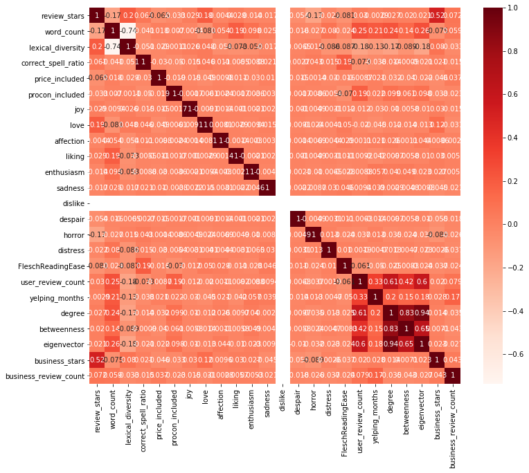
We found the strongest correlation (0.94) between degree and eigenvector. The degree and betweenness are also strongly correlated (0.83). These results represent redundancies in attributes. We can drop one or two of them. However, we will leave it to the feature subset selection method in this exercise.

Data Integration 2

One common challenge in data integration is attribute construction. New attributes need to be constructed from the given ones if existing attributes do not adequately reflect the target label/value. For instance, the "area" is a better indicator of housing prices than the "length" and "width" of a house. We observed that attributes related to sentiment are sparse. Most of them are zeros. We will create new attributes from the given ones. The attributes in the left of the arrow mark are existing ones, and the attributes in the right are new ones.

  • joy, love, affection, liking, enthusiasm -> positive_emotion
  • sadness, dislike, despair, horror, distress -> negative_emotion
yelp_data["positive_emotion"] = yelp_data["joy"] + yelp_data["love"] + yelp_data["affection"] + yelp_data["liking"] + yelp_data["enthusiasm"]
yelp_data["negative_emotion"] = yelp_data["sadness"] + yelp_data["dislike"] + yelp_data["despair"] + yelp_data["horror"] + yelp_data["distress"]

## Drop existing attributes
yelp_data = yelp_data.drop(["joy", "love", "affection", "liking", "enthusiasm", "sadness", "dislike", "despair", "horror", "distress"], 1)    

print(yelp_data.head())
                review_id  review_stars  word_count  lexical_diversity  \
0  bRGHgwAd3zfiiDMT9JyKcA             1          23           0.869565   
1  TK-0pfhHorvwZK0YhDe2fQ             5          26           0.769231   
2  XTOQ6blQzzzoK26QRJl3zg             5          71           0.760563   
3  KA9VwKYL-7I2LuQnXeuEBw             5          74           0.689189   
4  C2kblEfR4oMWR9oGhYN2cQ             5          31           0.903226   

   correct_spell_ratio  price_included  procon_included  FleschReadingEase  \
0             0.869565        0.000000                0            81.1310   
1             0.846154        0.000000                0            48.9568   
2             0.943662        0.014085                0            95.9393   
3             0.905405        0.000000                0            86.9222   
4             0.903226        0.000000                0            63.0018   

   user_review_count  yelping_months  degree  betweenness  eigenvector  \
0                  5              24       0          0.0          0.0   
1                 22               6       1          0.0          0.0   
2                 10              14       0          0.0          0.0   
3                  1               3       0          0.0          0.0   
4                 19              40       0          0.0          0.0   

   business_stars  business_review_count       class  positive_emotion  \
0             3.0                     40      useful               0.0   
1             4.5                    319      useful               0.0   
2             4.5                    535  not_useful               0.0   
3             5.0                     28      useful               0.0   
4             3.5                     84      useful               0.0   

   negative_emotion  
0               0.0  
1               0.0  
2               0.0  
3               0.0  
4               0.0  

Dimensionality Reduction + Normalization

As a method of data reduction, we can apply dimensionality reduction. We covered PCA and feature subset selection in the lecture. In this exercise, we will cover feature subset selection. We are also going to apply normalization before selecting a feature subset. We will implement the forward selection and bi-directional stepwise selection.

## Create feature matrix by dropping the review_id and label attribute
## Review_id is not going to helpful to predict the usefulness of reviews
X = yelp_data.drop(["review_id","class"], 1)    

## Pre-processing. Sklearn takes integer as label
# ## Create target attribute
yelp_data[yelp_data['class'] == 'useful'] = 1
yelp_data[yelp_data['class'] == 'not_useful'] = 0

# ## Specify the data type. Before specifying, the type was unknown
y = yelp_data["class"].astype('int')

print(yelp_data["class"])
0      1
1      1
2      0
3      1
4      1
      ..
995    1
996    1
997    1
998    0
999    1
Name: class, Length: 998, dtype: int64
print(X.shape[1])

## import the necessary libraries
from mlxtend.feature_selection import SequentialFeatureSelector as SFS
from sklearn.naive_bayes import MultinomialNB
from sklearn import preprocessing

## Apply Min_Max Scaler
min_max_scaler = preprocessing.MinMaxScaler()
X_minmax = min_max_scaler.fit_transform(X)
X_minmax = pd.DataFrame(X_minmax)

## Sequential Forward Selection(sfs)
## Please refer to http://rasbt.github.io/mlxtend/user_guide/feature_selection/SequentialFeatureSelector/#sequential-feature-selector
## for the detailed arguments options
sfs = SFS(MultinomialNB(),
           k_features=(1,X_minmax.shape[1]),
           forward=True, 
           floating=False,
           scoring = 'r2',
           cv = 10)

sfs.fit(X, y)
## Get the final set of features
sfs.k_feature_names_     
16
('review_stars',
 'word_count',
 'lexical_diversity',
 'correct_spell_ratio',
 'price_included',
 'procon_included',
 'FleschReadingEase',
 'degree',
 'betweenness',
 'eigenvector',
 'business_stars',
 'positive_emotion',
 'negative_emotion')
from mlxtend.plotting import plot_sequential_feature_selection as plot_sfs
import matplotlib.pyplot as plt

## performance graph (y-axis: r-squared values)
fig = plot_sfs(sfs.get_metric_dict(), kind='std_dev')
plt.title('Sequential Forward Selection (w. StdErr)')
plt.grid()
plt.show()

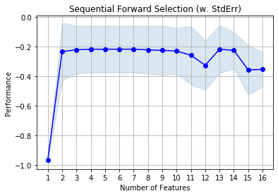
Thirteen attributes were selected. Let's try bi-directional stepwise selection (combination of forward and backward selection) and compare results.

## Bi-directional stepwise selection
## Please note that floating option was changed to "True"
sfs1 = SFS(MultinomialNB(),
           k_features=(1,X_minmax.shape[1]),
           forward=True, 
           floating=True,
           scoring = 'r2',
           cv = 10)

sfs1.fit(X, y)
# Get the final set of features
sfs1.k_feature_names_     
('review_stars',
 'word_count',
 'correct_spell_ratio',
 'price_included',
 'eigenvector',
 'positive_emotion',
 'negative_emotion')
## performance graph (y-axis: r-squared values)
fig1 = plot_sfs(sfs1.get_metric_dict(), kind='std_dev')
plt.title('Sequential Bi-directional Stepwise Selection (w. StdErr)')
plt.grid()
plt.show()

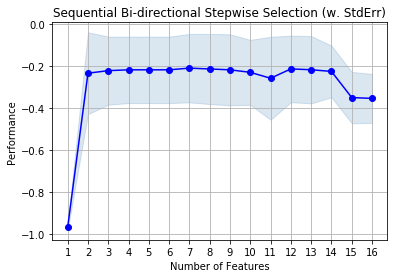
Now, we have seven attributes ('review_stars','word_count','correct_spell_ratio','price_included','eigenvector','positive_emotion','negative_emotion'). We have a reduced set of attributes. The performance from both selection methods seems to be not very different. Potentially, using a small set will be better if the performance is not very different? However, it is still early to conclude. We did not separate data into training and testing sets. Also, what is the goal of your classifier? Is it effectiveness or efficiency? Usually, we need to sacrifice one to achieve another. In other words, effectiveness increases when efficiency decreases, and vice versa. We will cover these topics later.