

Many machine learning problems in the real world cannot be solved by a linear equation. Consider the car evaluation data in the following table:
| Buying Price | Maintenance Cost | Evaluation |
|---|---|---|
| 2 | 2 | Acceptable |
| 2 | 1 | Acceptable |
| 1 | 2 | Acceptable |
| 1 | 1 | Acceptable |
| 4 | 4 | Unacceptable |
| 4 | 3 | Unacceptable |
| 4 | 2 | Unacceptable |
| 4 | 1 | Unacceptable |
| 3 | 4 | Unacceptable |
| 3 | 3 | Unacceptable |
| 3 | 2 | Unacceptable |
| 3 | 1 | Unacceptable |
| 2 | 4 | Unacceptable |
| 2 | 3 | Unacceptable |
| 1 | 4 | Unacceptable |
| 1 | 3 | Unacceptable |
Buying price and maintenance cost are on a scale of 1 to 4, with 1 meaning the lowest price (cost) and 4 the highest.
In the data, the concept is about whether a car is acceptable or unacceptable given its buying price and maintenance cost.3 The price (cost) variables are on an ordinal scale: low, medium, high, and very high, which we convert into an equal-interval numeric scale from 1 (low) to 4 (very high).
While it is possible to include other variables such as the number of doors and safety features, we will focus on the cost factors in the discussion here. The figure plots maintenance cost vs. buying price, with the $+$ indicating an acceptable car and $\circ$ unacceptable. The two classes appear not separable linearly on the two-dimensional space – that is, there is no straight line that can be drawn to separate the two.
Again, if one can introduce other predictor variables and the classes might be separable linearly on a higher-dimensional space. But even with the only two variables, namely maintenance cost and buying price, the plot seems to suggest that a car will be evaluated unacceptable with either a high buying price or a high maintenance cost.
Perhaps one can draw two straight lines, one to separate the classes on the price dimension and the other on the maintenance cost. However, this is no longer one linear equation of the two variables that can fit in with a linear model. Alternatively, we can still draw a curve (a non-linear function) to separate them. For example, as shown as the dashed line, a circular function such as $(v_1-1)^2 + (v_2 -1)^2 = 3$ can set the boundary between the two classes. The question is: how can we identify such as a non-linear function from the training data?
We have discussed the support vector machines, which, in its original form, is a linear model. How can we apply SVM to non-linear data? Now instead of finding out a non-linear function, we can think about how the data can be transformed in such a way that they are linearly separable.
In particular, we can map the data onto a higher dimensional space with richer features, where a linear classifier is applicable. Now that we do not have additional variables, how can we create a higher-dimensional space? The basic idea is to find non-linear combinations of existing variables, via a so-called kernel function. We will have an in-depth discussion of kernel functions in Chapter . But in the nutshell, a kernel function can be computed by a dot product with expanded features and makes it extremely efficient to identify the decision hyperplane in the higher dimensional space.
Among families of kernel functions, a polynomial function is often used. For example, we may consider a quadratic transformation with the car evaluation data.
Given the two existing variables, any data instance with $v = (v_1, v_2)$ (a two-dimensional vector) can be expanded onto a vector with more dimensions such as:
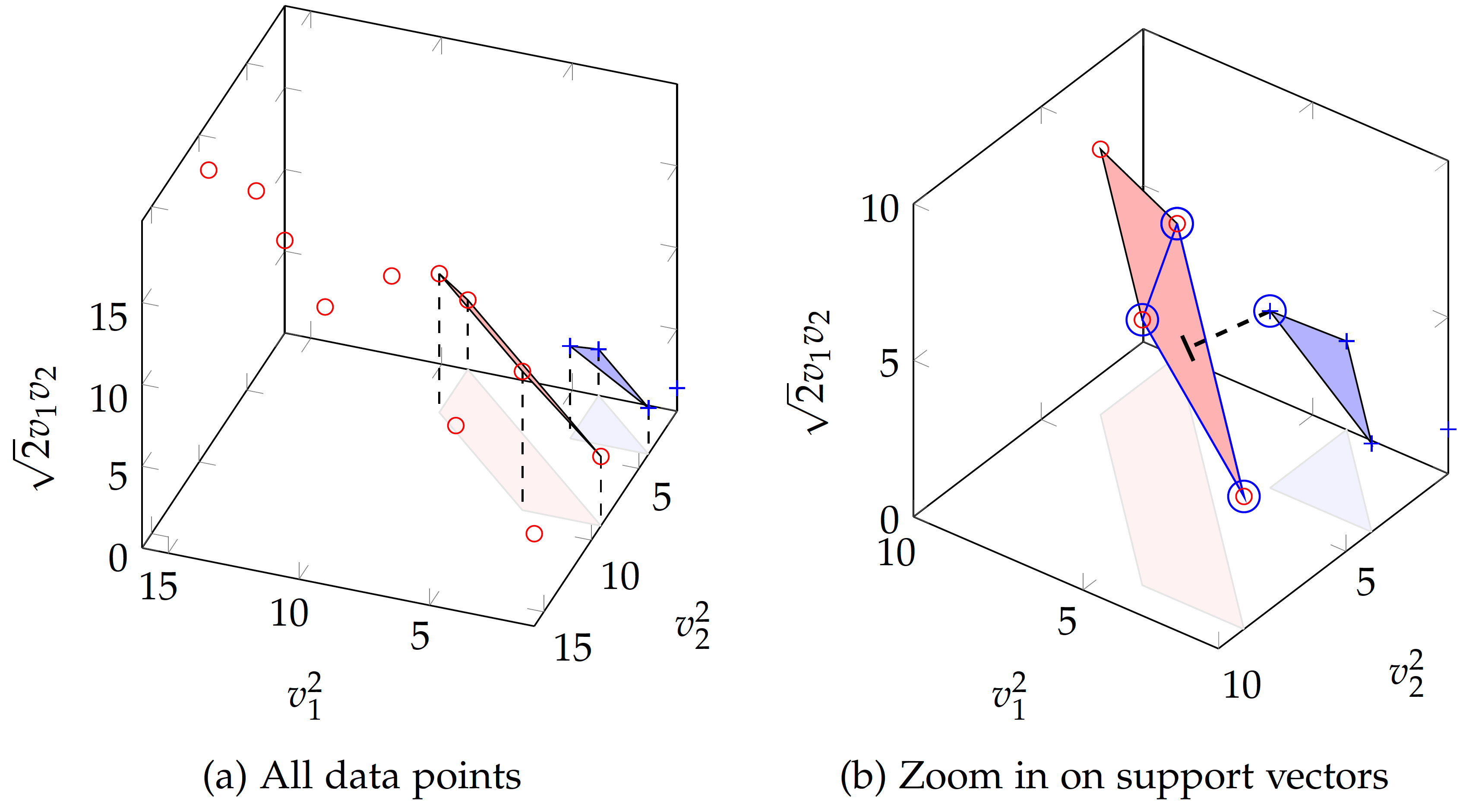
\begin{eqnarray} \phi(v) & = & (v_1^2, v_2^2, \sqrt{2} v_1 v_2)\end{eqnarray}Note that the quadratic expansion should result in 5 dimensions including the original dimensions of $v_1$ and $v_2$. We focus on the 3 additional features and thus limit the number of dimensions to three, which can be visualized.
Linear equation of $(v_1^2, v_2^2)$ at $v_1^2+v_2^2-9=0$:
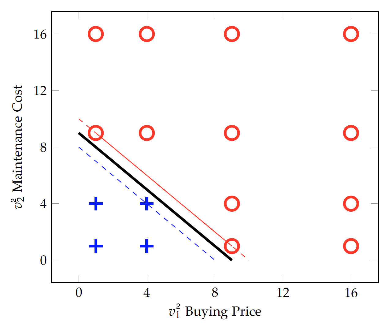
With the $v_1^2$ and $v_2^2$ transformation, data in the two classes already appear to be linearly separable. Again, they linear in the transformed data. As shown in the figure below, the solid line at $v_1^2+v_2^2-9=0$ can separate the data we have so far. However, this does not necessarily represent the general idea of car evaluation -- the boundary is rather narrow and new data may cross the decision boundary and violate the identified rule. The model is perhaps underfitting the data.
With the quadratic expansion, the additional dimension of $\sqrt{2} v_1 v_2$ can be seen as an interaction variable in the form of multiplication.
That is, whether a car is acceptable or not may depend on some form of interaction between the buying price and maintenance cost.
When all three expanded features are considered:
\begin{eqnarray} \phi(v) & = & (v_1^2, v_2^2, \sqrt{2} v_1 v_2) \end{eqnarray}the data are mapped to a three-dimensional space shown in the figure below, where they may be separated linearly. Of all linear equations (planes) formed by any three points in each class, we have identified two planes closest to their opposite classes.
Figure (a) shows all data points in the expanded dimensional space with quadratic mapping. The two planes formed by data points are the closest to the opposite class, which are candidate support vectors. Shadows of the planes are projected to the "ground" (i.e. $v_2^2$ vs. $v_1^2$ dimensions) for easier reading of related data points.
Figure (b) zooms in on the planes formed by candidate support vectors in the three-dimensional space, where a decision boundary can be identified to maximize the margin between the two classes (convex hulls). The dashed line connects the closest points of data in the two classes (convex hulls), by drawing a line from the circled positive point perpendicular to the plane formed by three circled negative points. The four circled points (one positive and three negative) are the identified support vectors, based on which the margin is established and classification can be performed.
Besides polynomial kernels, other popular kernel functions for SVM include radial basis and string kernels. A string kernel, for example, operates directly on symbol sequences without vectorized features and is useful in applications such as text classification and gene sequence analysis.
We know the single perceptron can only be applied to linearly separable data. The car evaluation data cannot be separated by one linear function. However, with a step function, one can transform the data into something linearly separable.
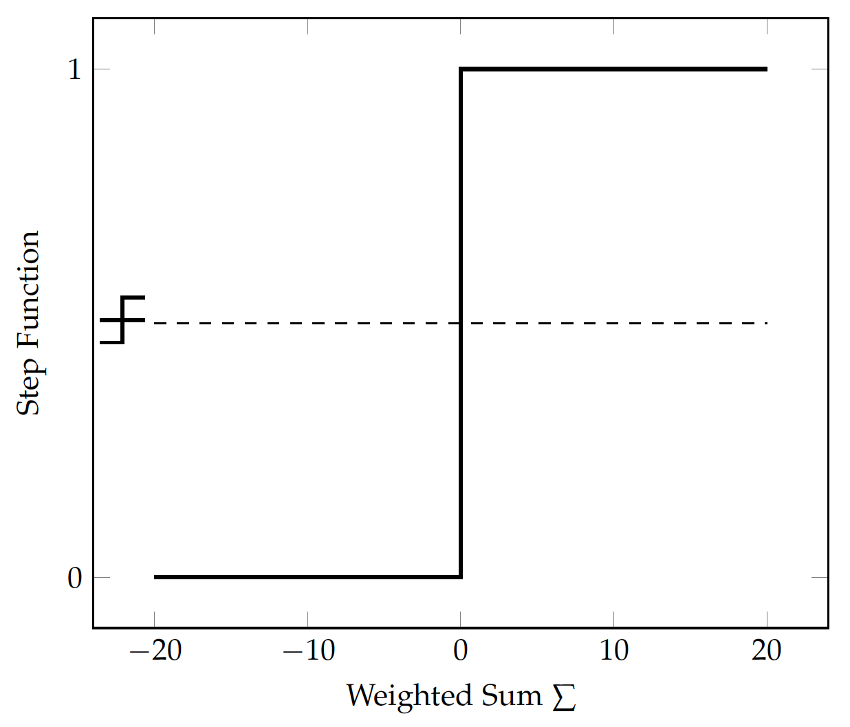
Specifically, for a value $v$ on the $v_1$ or $v_2$ dimension, we use the following step function:
\begin{eqnarray} f(v) & = & \begin{cases} 1 & \text{if}\ v>2.5\\ 0 & \text{otherwise} \end{cases}\end{eqnarray}Let $h_1 = f(v_1)$ and $h_2 = f(v_2)$:
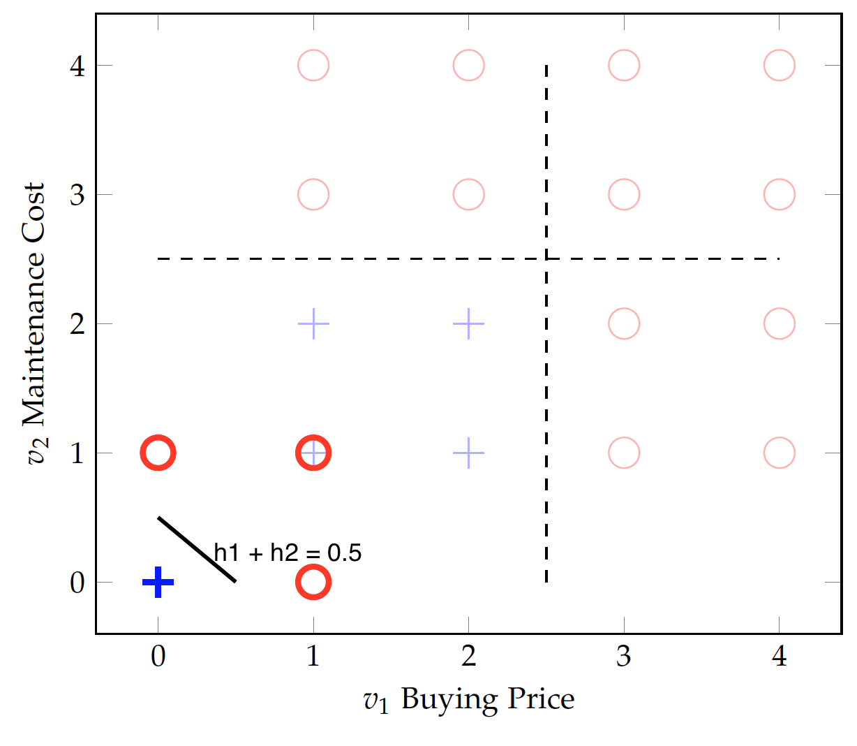
So it returns 1 for a value above 2.5, and 0 for a value below. Applying the step function to both $v_1$ (buying price) and $v_2$ (maintenance cost), we have transformed data in the above figure. All positive (acceptable) data have been mapped to the $(0,0)$ point whereas the negative (unacceptable) ones are at $(0,1)$, $(1,1)$, and $(1,0)$. As the solid line indicates, the transformed data are now linearly separable.
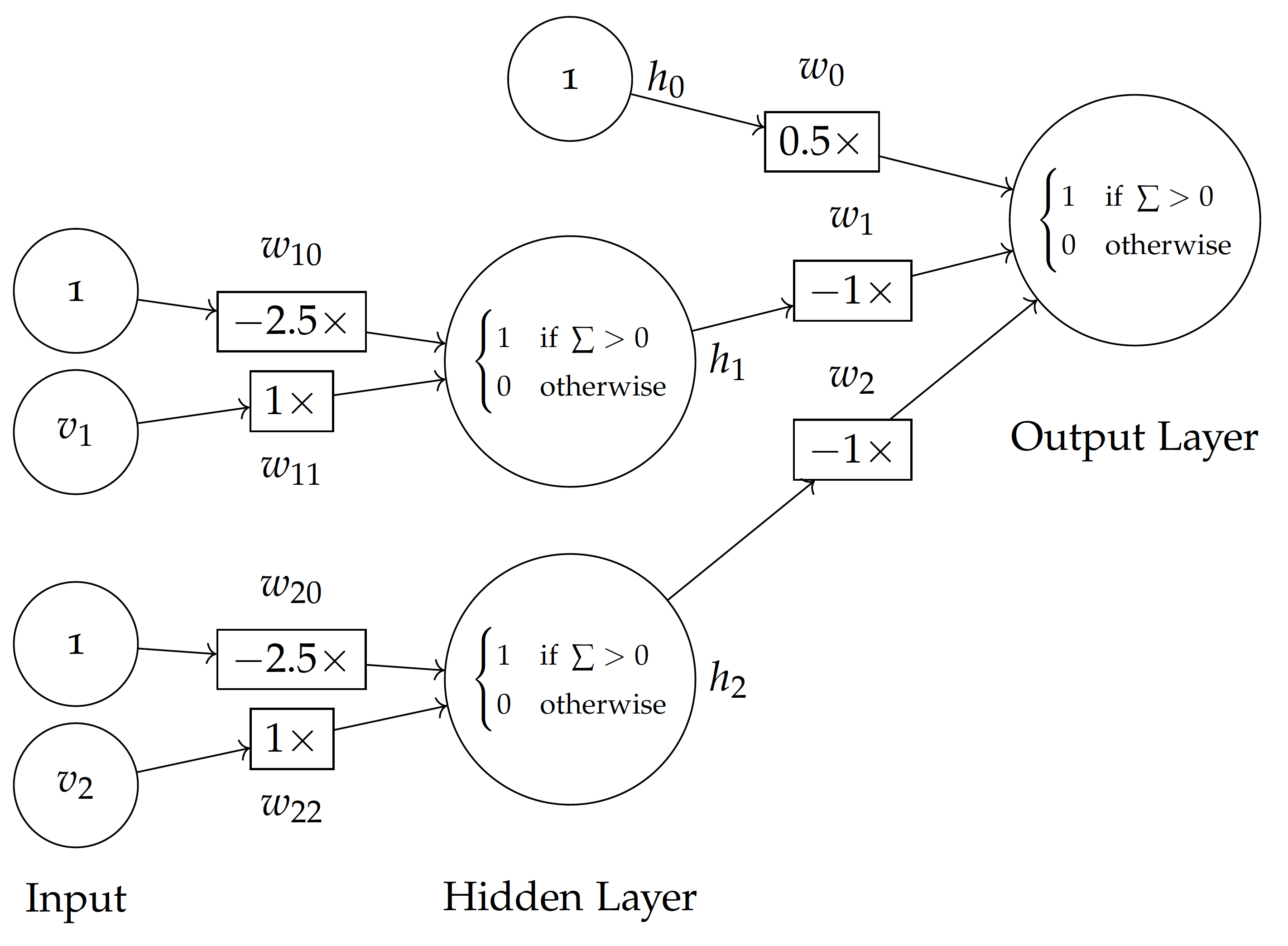
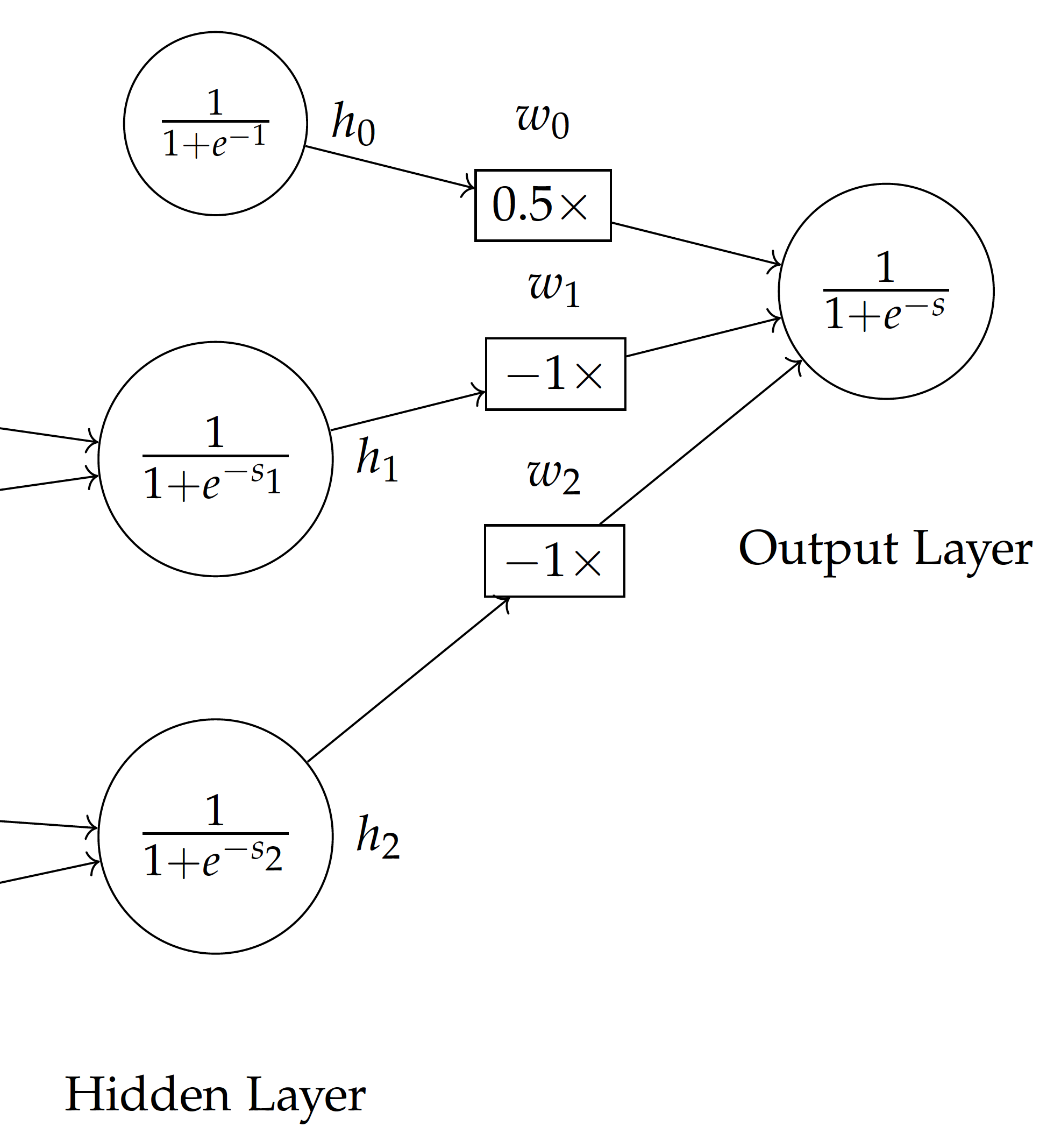
This non-linear classification with step function transformation can be represented with a multi-layer neural network. As shown in the figure here, each of the input variables $v_1$ and $v_2$ is normalized by a step function and then multiplied by $-1$ before feeding into the final output, which is combined with the bias weighted 0.5. This is equivalent to $0.5 \times 1 -1\times f(v_1) - 1\times f(v_2)$, where f is the step function for $v_1$ and $v_2$ values.
For example, with data point $(2,2)$, the step function will convert the values into $(0,0)$. With the bias $0.5\times1$, the weighted sum is $0.5\times1 - 1\times 0 - 1\times 0 = 0.5$ and it will be classified positive (acceptable). With data point $(3,1)$, it is transformed into $(1,0)$ by the step function and the final weighted sum is $0.5\times1 - 1\times 1 - 1\times 0 = -0.5$, which will be classified negative (unacceptable).
Using the multi-layer neural network, based on the additional hidden layer with step functions between the input and final output, it is now possible to establish a non-linear model such as the one in the above figure.
But the question remains –
How can the weights of the model, together with the step function, be identified properly?
While it is tempting to use a similar strategy as with the single perceptron, the non-linearity of the model rules out such a linear strategy for weight adjustment.
Simply adding or subtracting weights (linear combinations) does not help when the model is non-linear.
Can we adjust the weights in a non-linear manner during training? In other words, can we adjust the weights based on how much each variable contributes to the final output via the hidden layer?
The general optimization technique called gradient descent makes it possible to find optimal values (weights) by searching in the derivatives of related functions.
However, a step function, as illustrated below, has a sudden jump (not smooth transition) between 0 and 1 and is not differentiable.
If we are to retain the idea of a step function, can we develop one that functions in the like manner and yet smooth and differentiable?
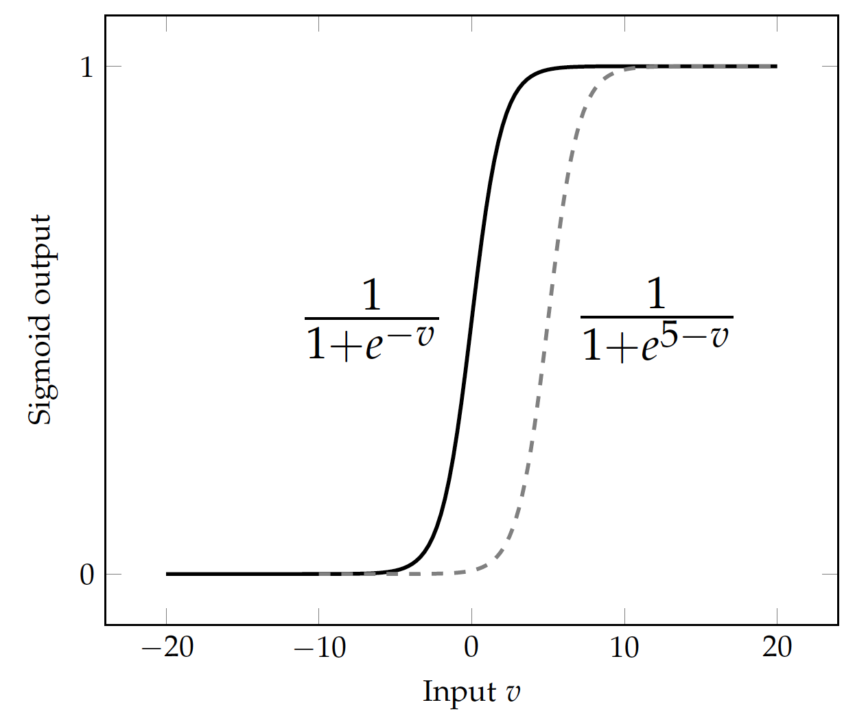
A candidate is the sigmoid function, which, for a value $v$, is defined by:
Or more generally:
\begin{eqnarray} f(v) & = & \frac{1}{1+e^{k-v}} \end{eqnarray}where $k$ is the pivot value
The figure here shows the functional curve of sigmoid, which transforms the weighted sum of a node to a value approaching 0 or 1. The threshold or pivot is 0 by default but we can use any threshold for the transformation.
For example, with a pivot value $k = 5$, the sigmoid function becomes:
\begin{eqnarray} f(v) & = & \frac{1}{1+e^{5-v}}\end{eqnarray}which shifts the functional curve on the x coordinates by +5 (dashed line in the above figure). $v-5 = 1\times v + (-5)\times 1$ is equivalent to the weighted sum of variable $v$ (with weight $w=1$) and bias $1$ (with weight $w_0=-5$). It can be generalized as a linear function of any number of input variables with bias in the form of $\sum = w_0 + \sum_i w_i v_i$.
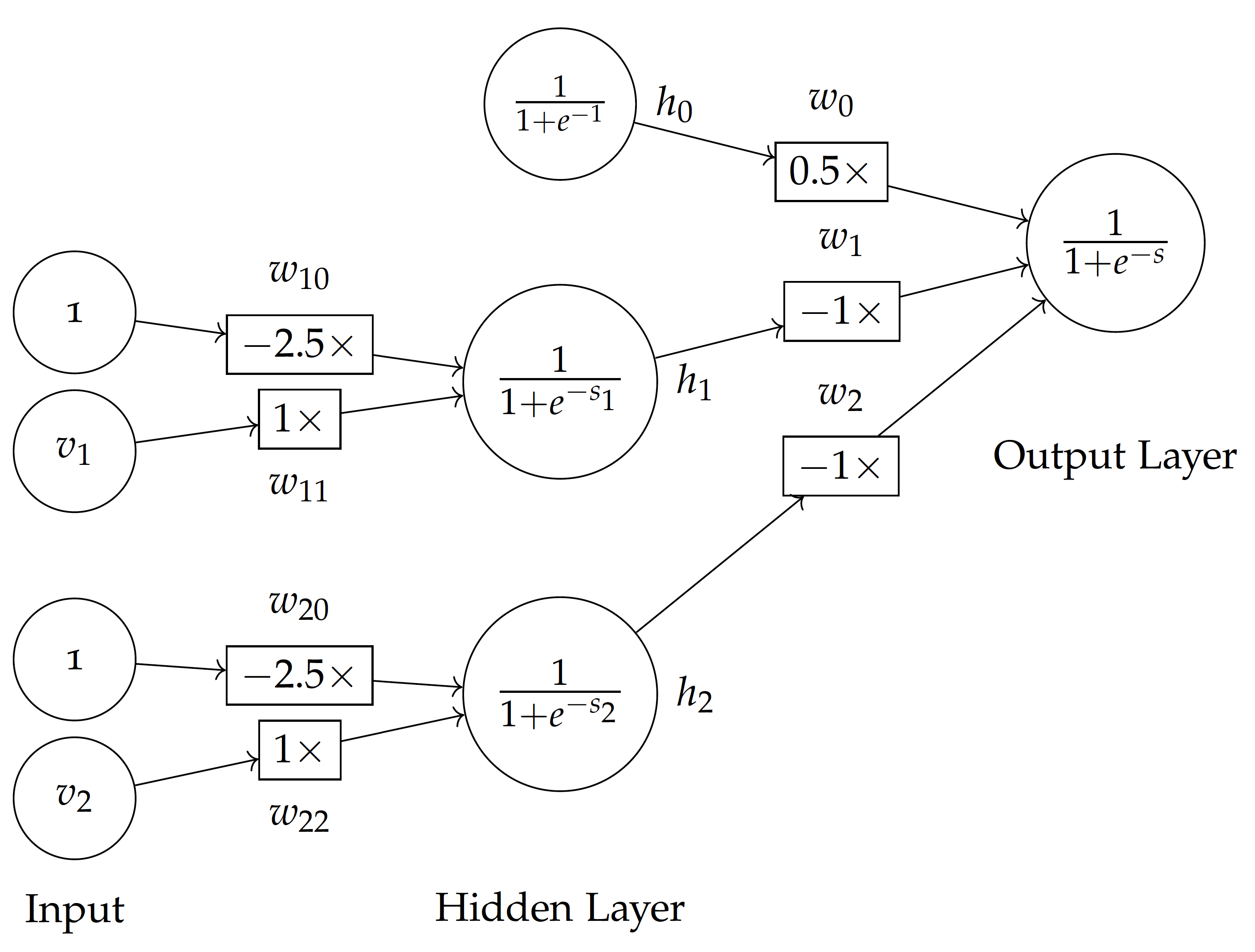
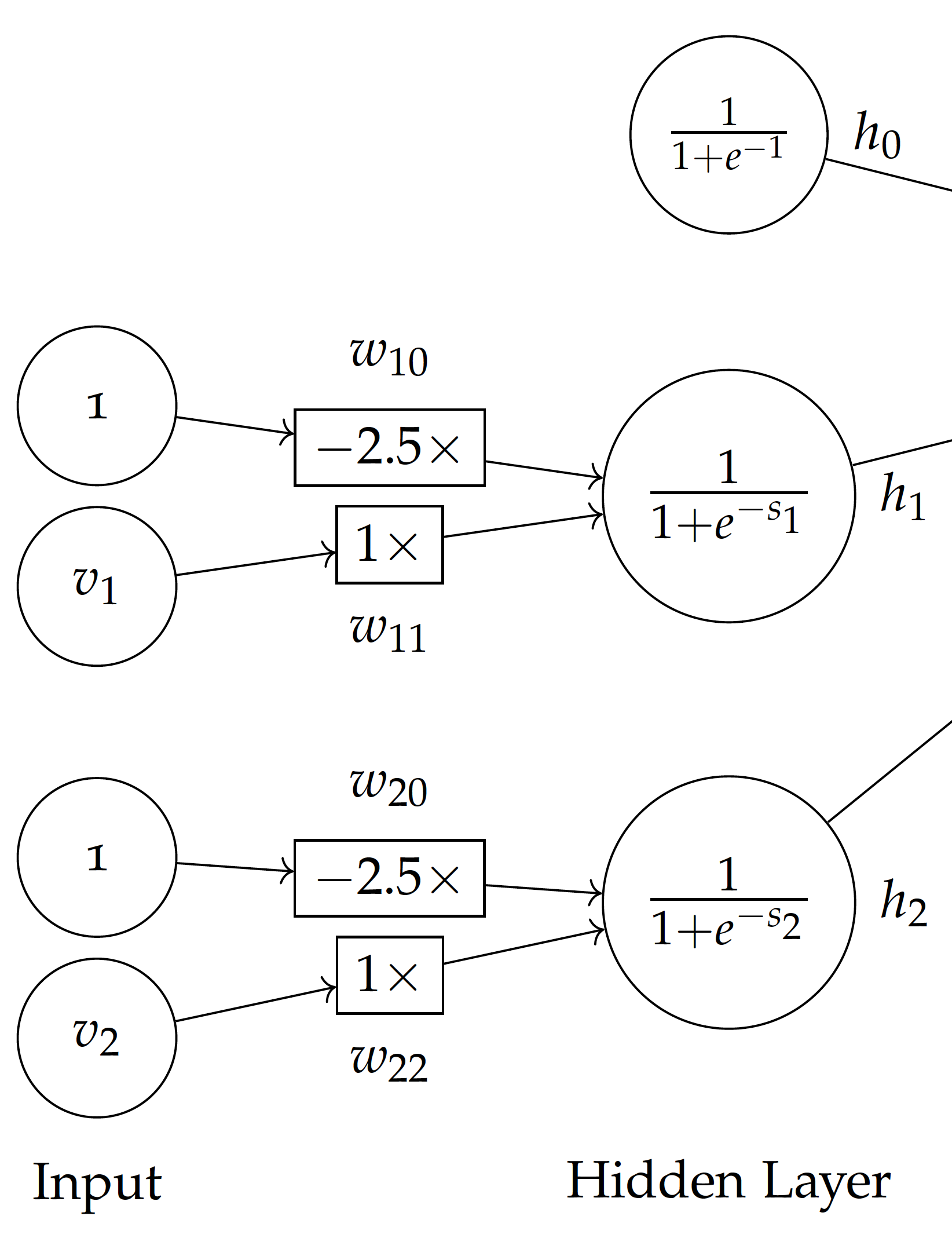
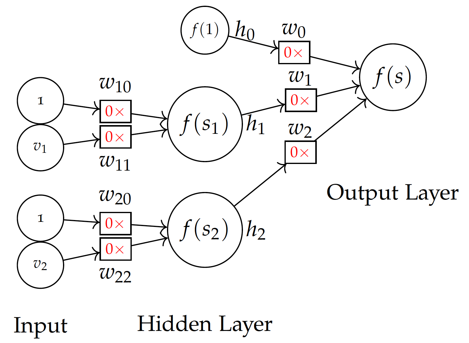
Now if we replace the step function with the sigmoid function, we have a multi-layer neural network shown above, in which each layer (node) is differentiable and the weight can be learned from a process such as gradient descent.
where
- $m$ is the number of variables
- $v_0$ is the bias, which is always 1
Given the sigmoid function $f$, the output of each node in the hidden layer is:
In light of the nerual network here, this can be written as:
The final output, predicted value $\hat{y}$, is the sigmoid of the weighted sum of values from the hidden layer $h$ values:
Again, for the model here, this can be computed by:
 \begin{eqnarray}
\hat{y}
& = & f(w_0 h_0 + w_1 h_1 + w_2 h_2) \\
& = & f\Big(w_0 f(1) \\
& & + w_1 f\big(w_{10} + w_{11} v_1 + w_{12} v_2\big) \\
& & + w_2 f\big(w_{20} + w_{21} v_1 + w_{22} v_2\big)\Big)\end{eqnarray}
\begin{eqnarray}
\hat{y}
& = & f(w_0 h_0 + w_1 h_1 + w_2 h_2) \\
& = & f\Big(w_0 f(1) \\
& & + w_1 f\big(w_{10} + w_{11} v_1 + w_{12} v_2\big) \\
& & + w_2 f\big(w_{20} + w_{21} v_1 + w_{22} v_2\big)\Big)\end{eqnarray}
Let $y$ be the actual outcome (class 0 or 1) for the data instance.
We define the error E as a squared function:
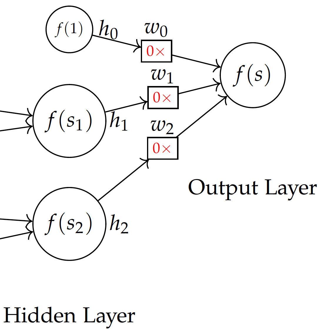
\begin{eqnarray} E(h) & = & \frac{1}{2} (y - \hat{y})^2\end{eqnarray}For a prediction based on the sigmoid function $f$, it can be shown that the differential with respect to a weight $w_i$ to the output layer is:
where $s$ is the weighted sum to the output layer and $f'(s)$ is the derivative of the sigmoid function $f(s)$, which is as simple as $f(s)(1-f(s))$. This gives the differentials needed to optimize $w_i$ weights from the hidden layer to the output, i.e. $w_0$, $w_1$, and $w_2$ weights in the model here.
The differentials will be used to update weights to both layers during the training process. In particular, the differential $\frac{dE(h)}{dw_i}$ will be used to subtract from existing weights of $w_0$, $w_1$, and $w_2$.
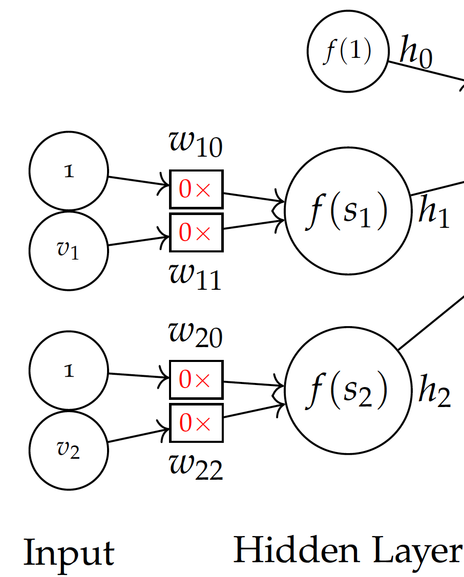
Now that values in the hidden layer $h$ are based on weighted sums of the input layer, we also need to optimize $w_{ij}$ weights connecting the input to the hidden layer.
Given input values $v$, the differential with respect to a weight $w_{ij}$ to hidden node $h_i$ can be computed by:
where:
- $f'(s) = f(s)(1 - f(s))$
- $f'(s_i) = f(s_i)(1 - f(s_i))$
The differential $\frac{dE(v)}{dw_{ij}}$ will be used to subtract from existing weights of $w_{10}$ and $w_{11}$ for $h_1$; $w_{20}$ and $w_{22}$ for $h_2$ in the model. This approach of revising weights to the two layers can thought of as propagating differentials of squared errors backward in the feed-forward neural network, and is referred to as backpropagation.
To understand how backpropagation actually operates, let’s walk through the training process with the first data instance in Table tab:bin:car_nn.
| Buying Price | Maintenance Cost | Evaluation |
|---|---|---|
| 2 | 2 | 1 |
| .. | .. | .. |
- 1 training instance for multi-layer neural network
- Evaluation value 1 for acceptable and 0 for unacceptable
Before training, we don’t know the weights and may initialize them with all 0 values. Note that we use 0 initial weights for easy demonstration. This is not necessarily the best strategy for initialization.
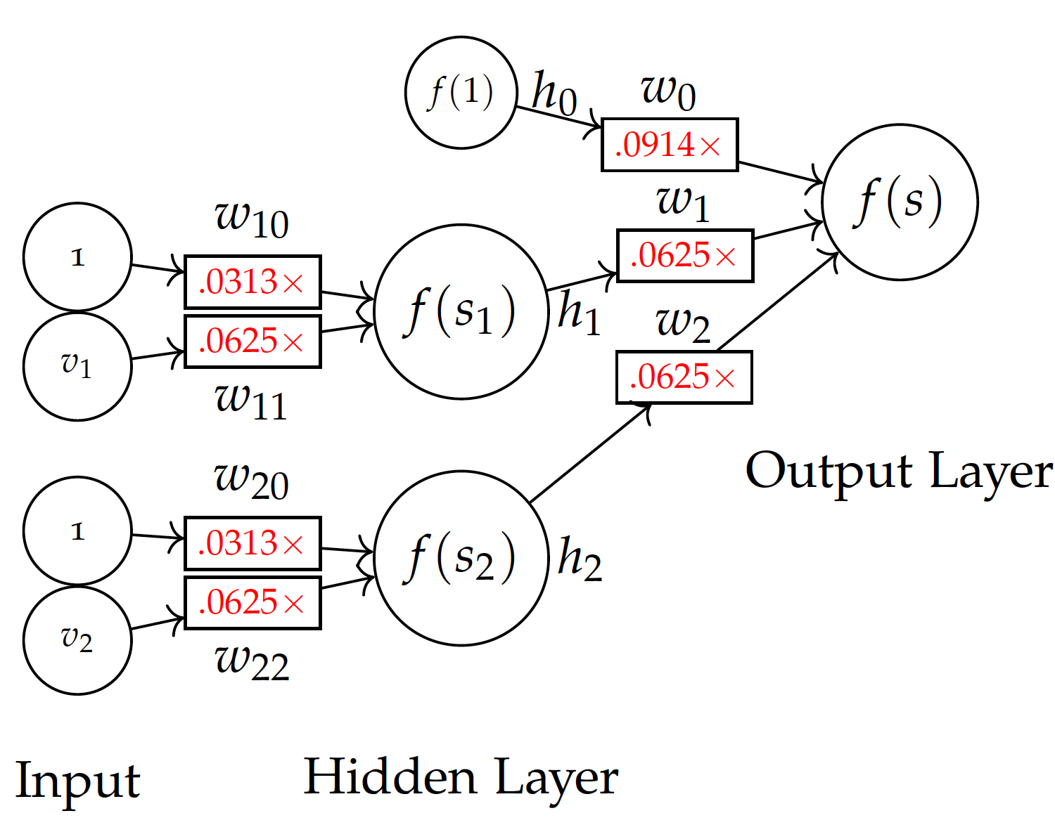
Backpropagation -- step 1 with 0 initial weights:
Now with the model and initial weights in the initial model, given the first training instance of (2,2), we can compute:
The final prediction $\hat{y}$ is computed by:
We get:
\begin{eqnarray} \big( f(s) - y \big) f'(s) & = & \big( f(s) - y \big) f(s) \big( 1 - f(s)\big) \\ & = & (0.5 - 1) \times 0.5 \times (1 - 0.5) \\ & = & - 0.125\end{eqnarray}With the actual class being 1, we can compute the differentials.
For each $w_i$ weight leading to the output layer:
\begin{eqnarray} \frac{dE(h)}{dw_0} & = & \big( f(s) - y \big) f'(s) h_0 \\ & = & -0.125 \times h_0 \\ & = & -0.125 \times 0.73 \\ & = & -0.0914 \\ \frac{dE(h)}{dw_1} & = & -0.125 \times 0.5 \\ & = & -0.0625 \\ \frac{dE(h)}{dw_2} & = & -0.0625 \\\end{eqnarray}Subtracting these (negative) values from their current weights respectively, we obtain the new weights $w_0=0.0914$, $w_1=0.0625$, and $w_2 = 0.625$.
Now we can further back-propagate the error to the $w_{ij}$ weights from the input layer:
Subtracting these from current $0$ values, we obtain new weights for of all $w_{ij}$, namely $w_{10}=0.0313$ and $w_{11}=0.0625$ to hidden node $h_1$, and $w_{20}=0.0313$ and $w_{22}=0.0625$ for hidden node $h_2$.
Backpropagation step 2 with updated weights:
The figure here shows the model with updated weights after training by the first instance $(2,2)$ with a known class label 1. We can continue to train the model with additional instances in car evaluation data. This can be repeated with the same data until weights are stabilized and the error is reduced to a certain level.
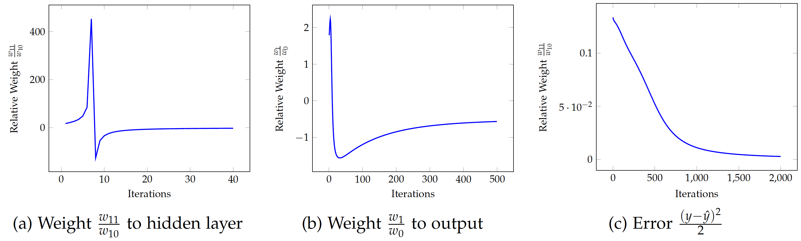
The figures show relative weights and error over time, via iterations of repeated training with data. Note that in linear equations, absolute values of related weights (coefficients) are not important. Rather, it is their relative weight to one another that matters. Hence, we present weights relative to $w_0$, i.e. divided by the bias weight.
Overall, the figures show the weights and error all appear to converge. However, they seem to differ in the number of iterations needed for their convergence. In Figure (a), the relative weight of $w_{11}$ (the weight of $v_1$ to the hidden node $h_1$) fluctuates a lot in the first 10 iterations but stabilizes quickly after a few dozen iterations. In Figure (b), $w_1$ – the weight from the hidden node $h_1$ to the final output – appears to take hundreds of iterations to converge. The squared error, as shown in Figure (c), takes even even more iterations to be minimized.
Converged model:
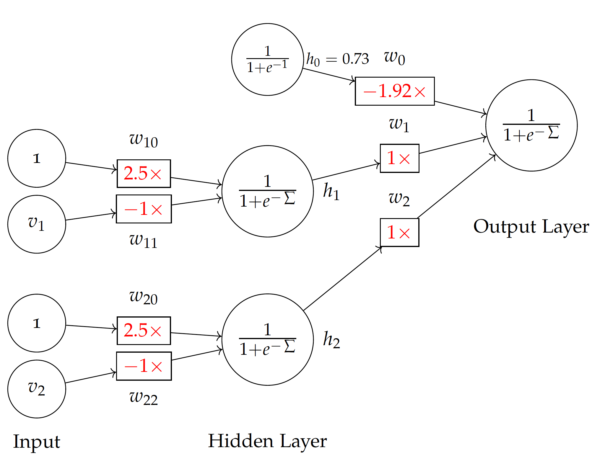
| Weights | $w_0$ | $w_1$ | $w_2$ | $w_{10}$ | $w_{11}$ | $w_{20}$ | $w_{22}$ | Error |
|---|---|---|---|---|---|---|---|---|
| Absolute | -18.4 | 9.47 | 9.44 | 7.35 | -2.93 | 7.43 | -2.96 | 0.0027 |
| Relative | -1 | 0.52 | 0.52 | 1 | -0.40 | 1 | -0.40 | 0.0027 |
| Relative | -1.92 | 1 | 1 | 2.5 | -1 | 2.5 | -1 | 0.0027 |
In the end, we obtain the weights in the above table with minimized squared errors. The result is highly similar to the model we illustrated earlier. For example, the weighted sum for hidden node $h_1$ is $2.5 - v_1$ in the model here, which is simply the negative of what is in the figure, where the sum is $v_1 - 2.5$. We observe the same with the hidden node $h_2$. This leads to the different signs of $w_1$, $w_2$ vs. $w_0$ to the output layer.
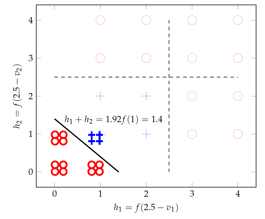
The plot here visualizes how the model transforms the original data into something separable. A sigmoid function with a weighted sum of $2.5 - v$ (for both $v_1$ and $v_2$) converts the original data (+ and $\circ$ in faded colors) to values close to 0 (if $v>2.5$) and 1 values (if $v<2.5$).
Given the limited training data we have, there are many non-linear solutions to the classification problem. In the end, we obtain the model here which is lightly different from what we proposed earlier. Both models will make perfect classifications on the simple training data presented in this lecture. However, a model thus obtained has not necessarily found the global optimal. In fact, the back-propagation mechanism via gradient descent can converge to a local optimum, which depends on many factors such as the starting point (initial values) and the sequence of training data. The learning rate also impacts the convergence of weights and, occasionally, may also influence where they converge.
A hyperplane in more three dimensions is hard to visualize. Mathematically, it shares the same functional form of Equation eq:bin:lin and is a natural extension of the lower-dimensional representation.
Please note additional data points than previously discussed in the illustration.
The tiny data set was inspired by the UCI’s Car Evaluation collection. However, this simplified version is intended for demonstration only and does not represent the actual data in the UCI repository.