
The notion of least action or least effort has long been observed in the natural world as well as human behavior. In spoken language, we tend to minimize our efforts by reusing old words and expressions, as if they are old tools meant for many applications. The results of this: words tend toward "a minimum in number and size" and "the older the tool (word) the more different jobs it can perform."
Under the Principle of Least Effort, there appears to be a great divide between a small number of words so frequently used and those rarely mentioned.
In particular, if we sort words by their frequencies, a term $t$’s frequency $f_t$ is proportional to the inverse of its rank $k_t$:
where word $t$ is ranked the $k^{th}$ most frequent.
This means, if you count the frequency of each word in a collection of text collection:
| Rank $k_t$ | Word $t$ | Frequency $f_t$ | $\propto \frac{1}{k_t}$ |
|---|---|---|---|
| 1 | the | 1,000,000 | $ \propto \frac{1}{1}$ |
| 2 | be | 500,000 | $ \propto \frac{1}{2}$ |
| 3 | to | 333,000 | $ \propto \frac{1}{3}$ |
| 4 | of | 250,000 | $ \propto \frac{1}{4}$ |
| .. | .. | ... | ... |
| k | $k_t$ | $\frac{10^6}{k_t}$ | $ \propto \frac{1}{k_t}$ |
If we consider probabilities rather than raw frequencies, the above can be written as:
where $c$ is a constant. In the English language, empirical data have shown $p(t) \approx 0.1 / k_t$ within the top $1,000$ rank, which means:
| Rank $k_t$ | Word $t$ | Probability $p(t)$ | $= \frac{c}{k_t}$ |
|---|---|---|---|
| 1 | the | 0.100 | $ \approx \frac{0.1}{1}$ |
| 2 | be | 0.050 | $ \approx \frac{0.1}{2}$ |
| 3 | to | 0.033 | $ \approx \frac{0.1}{3}$ |
| 4 | of | 0.025 | $ \approx\frac{0.1}{4}$ |
| .. | .. | ... | ... |
| k | $k_t$ | $\frac{10^6}{k_t}$ | $ \approx \frac{0.1}{k_t}$ |
This relation can be visualized in the figure here:
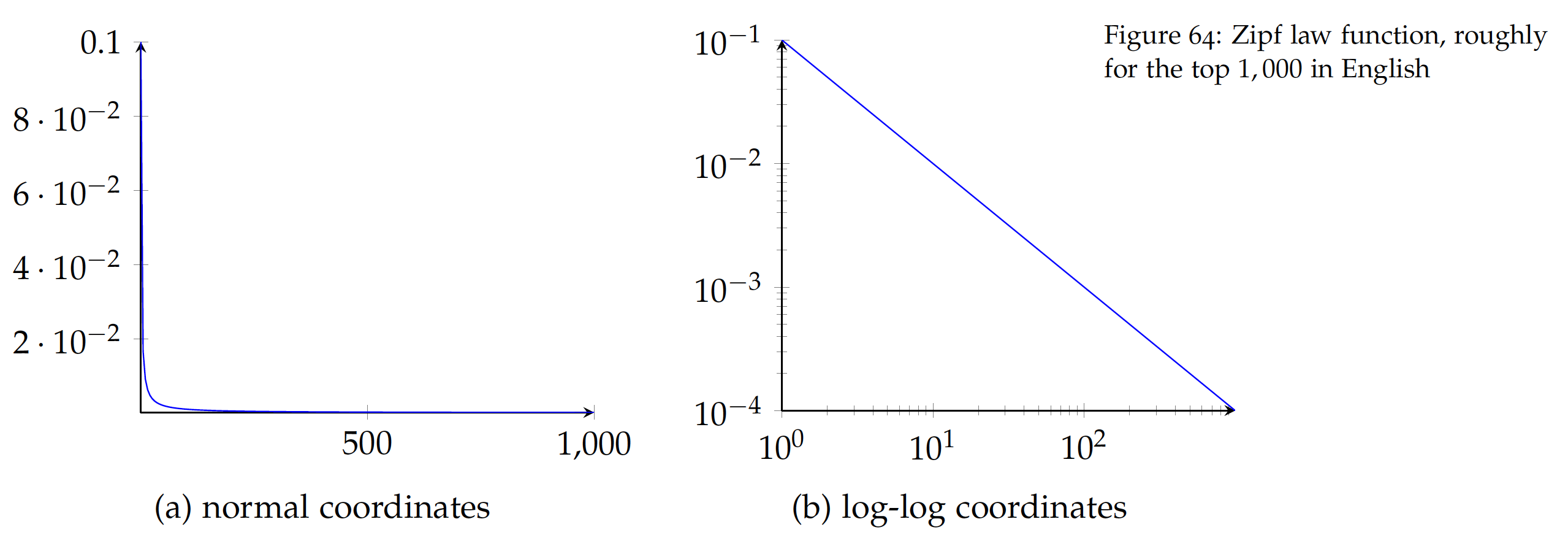
With a long tail, Figure (a) on normal coordinates is difficult to examine and it is often useful to apply the logarithmic transformation. By taking the log of both x (rank) and y (frequency) values, this can be transformed into Figure (b). As shown, Zipf law is a linear function on log-log coordinates and is a special case of power-law distributions, which, as we discussed in Chapter , are results of the Matthew effect (the rich get richer). In fact, there is an intrinsic connection between the Principle of Least Effort and the Matthew effect – as we tend to a minimum set of vocabulary, what we have frequently used (old "rich" words) will be used even more frequently (richer).
We have observed that any text processing may involve a very large number of features (terms) and it is a common practice to perform feature selection in such processes as clustering, classification, and retrieval (search).
In light of Zipf’s law, there are a large number of words that are rarely used, only in a few documents. While these terms might be informative when they occur, their rare occurrences make them less useful in such tasks as clustering and classification where documents are grouped by terms they have in common. Given that there are many low frequent words – the long tail of the Zipf function – removing them will reduce the dictionary size (feature space) significantly.
In terms of document frequency (DF), on the other hand, we know highly frequent words such as stop words are not informative and can be safely removed in certain applications. In practice, simple feature selection techniques such as DF (document frequency) thresholding has performed very effectively with little computational cost. It has been shown that having the right number of features is key to the success of text clustering and classification – using all features not only slows down the processing but also contributes more noise than information for related tasks.
With a distance or similarity measure in the vector representation, it is now possible to compare documents to one another and associate them with data groups or labels. For example, one may use an instance-based lazy learning method such as kNN with cosine similarity to perform classification and prediction based on the nearest data vectors.
Another successful approach is to model the probability that a document belongs to each class (label) and assign the document to the class that maximizes the probability. That is, given a document representation d, we need to estimate the probability of each class p(c_i|d), where c_i is one of the given classes to be predicted.
Say we are working on email spam filtering based on subject titles. This is a binary classification problem, for which we have two classes (labels) – an email is either a ham (normal) or a spam (junk). Suppose we have a small collection of email subjects which we have labeled ham or spam to train our model (learning):
| DOC | Email Subject | Class |
|---|---|---|
| 1 | You have been selected! | spam |
| 2 | Have a prize for you! | spam |
| 3 | You won! | spam |
| 4 | Project meeting schedule | ham |
| 5 | Nice to meet you! | ham |
| 6 | Project update | ham |
| 7 | Update on research | ham |
Given the short subject titles, let us first look at how we can model probabilities in text if we only consider binary occurrences of terms. Assume we remove some of stop-words (e.g. have, been) and normalize some others (e.g. meeting $\to$ meet, won $\to$ win), we can represent the email using the following dictionary:
| 1 | 2 | 3 | 4 | 5 | 6 | 7 | 8 | 9 | 10 | ||
|---|---|---|---|---|---|---|---|---|---|---|---|
| DOC | meet | nice | prize | project | research | schedule | select | update | win | you | Class |
| 1 | 1 | 1 | spam | ||||||||
| 2 | 1 | 1 | spam | ||||||||
| 3 | 1 | 1 | spam | ||||||||
| 4 | 1 | 1 | 1 | ham | |||||||
| 5 | 1 | 1 | 1 | ham | |||||||
| 6 | 1 | 1 | ham | ||||||||
| 7 | 1 | 1 | ham | ||||||||
Within a class $c$, there is a probability that a term $t$ will occur in a (random) document $p(t|c)$. To estimate the probability, one can simply count the ratio between the number of emails t appears and the total number of emails in class c.
However, as we discussed in Chapter , this approach may lead to skewed estimates and potential zero probability values due to data variance in the sample. Now that we have a very small data set here, we will use the Laplace estimator with an added constant \mu to any count, that is:
where $n(t|c)$ is the number of documents in class c that contain term t (document frequency) and N(c) is the total number of documents belonging to c. $\mu$ is a constant added to avoid zero probability estimates and $2\mu$ in the denominator is to account for $\mu$ being added to the binary cases (for when $t$ occurs and when it does not).
For example, with $\mu=0.05$, some of the term probabilities in the spam class can be computed by:
The same probabilities in the ham class are:
In the binary representation, w_t = 1 when term t occurs in the document and w_t = 0 if it does not. Given p(t|c) probability term t occurs in a (random) document in class c, 1 - p(t|c) is the probability that it does not occur.
That is, the probability of observing a binary term weight w_t can be written as the Bernoulli probability mass function:
For term prize in the spam class, the above can be written as:
Similarly, probability of a term weight for you in the ham class:
Following this, we can estimate the probability of any term weight $w_t$ in the classes ham vs. spam.
Now suppose we receive a new email and try to determine whether it is a ham or a spam:
| DOC | Email Subject | Class |
|---|---|---|
| d | Your prize! | ? |
The new email to be classified can be represented as:
| 1 | 2 | 3 | 4 | 5 | 6 | 7 | 8 | 9 | 10 | ||
|---|---|---|---|---|---|---|---|---|---|---|---|
| DOC | meet | nice | prize | project | research | schedule | select | update | win | you | Class |
| d | 1 | 1 | ? | ||||||||
The question here is how we can estimate the probability of the email d being ham or spam, p(ham|d) vs. p(spam|d). Using the Bayes theorem, they can be computed by:
Both equations above have p(d) as the denominator, which does not affect the ratio of the two values (classification outcome) and can be ignored in the calculation.
p(ham) and p(spam) can be estimated by counting the number of hams vs. spams. With a Laplace estimator and $\mu=0.05$, they are:
For p(d|spam), email d can be viewed as a collection of its term weights w_t. Given the 10 terms in the dictionary, p(d|spam) is their joint probabilities p(w_t|spam) in the spam class.
Assume the term probabilities are independent (naive assumption), the conditional probability can be computed by:
| 1 | 2 | 3 | 4 | 5 | 6 | 7 | 8 | 9 | 10 | ||
|---|---|---|---|---|---|---|---|---|---|---|---|
| DOC | meet | nice | prize | project | research | schedule | select | update | win | you | Class |
| d | 1 | 1 | ? | ||||||||
Likewise, we can compute the probability conditioned on the ham class:
Plug the numbers back in Equations eq:text:nb_ham and eq:text:nb_spam, we have:
Clearly p(ham|d) < p(spam|d) and the new email d will be predicted as a spam.
Two important notes here. First, although the example only has two classes, the Naive Bayes classifier can be applied to more than two classes. Given a document d and a set of classes C = [c_1, c_2, .., c_k], where k \ge 2, the general Naive Bayes model with Bernoulli distribution is to identify a class \hat{c} such that the posterior probability p(c|d) is maximized:
To predict class $c$ with the greatest probability $p(c|d)$: \begin{eqnarray} \hat{c} & = & \arg \max_{c \in C} p(c|d) \\ & = & \arg \max_{c \in C} \frac{p(c)p(d|c)}{p(d)} \\ & = & \arg \max_{c \in C} \frac{p(c)\prod_{t} p(w_{dt}|c)}{p(d)}\end{eqnarray}
where $w_{dt}$ is the binary weight of term t in document d (to be classified). $p(d)$ is the common denominator for all classes and can be ignored in the calculation.
Second, the product of joint probabilities (with $\prod_t$ in the above equation) in the model can become a very small value, especially when there are a great number of terms in the dictionary. To avoid this computational difficulty, it is a better practice to convert this into a log-likelihood (by taking the logarithm of the probabilities):
In this way, we perform the addition of log-likelihood and can maintain a better precision with float points. Again $\log p(d)$ is a constant across the classes and can be omitted in the computing.
Now let us look beyond binary term occurrences for text classification. As we discussed earlier in the chapter, term frequency (TF) is a useful statistic, which we should also take advantage of in this task.
Suppose we extend the email representation from subject title to include email body (content) as well. Assume the dictionary (vocabulary) remains the same as in Table tab:text:emails_bin but obviously terms may occur multiple times in the email text.
The following is a hypothetical TF representation of the same emails:
| 1 | 2 | 3 | 4 | 5 | 6 | 7 | 8 | 9 | 10 | ||
|---|---|---|---|---|---|---|---|---|---|---|---|
| DOC | meet | nice | prize | project | research | schedule | select | update | win | you | Class |
| 1 | 1 | 3 | spam | ||||||||
| 2 | 3 | 2 | spam | ||||||||
| 3 | 2 | 2 | spam | ||||||||
| 4 | 2 | 1 | 3 | ham | |||||||
| 5 | 1 | 1 | 2 | ham | |||||||
| 6 | 2 | 1 | ham | ||||||||
| 7 | 3 | 1 | ham | ||||||||
The probability of term t in class c, p(t|c) can be computed by its overall term frequency (in all documents) over the total term frequency of documents in that class. Given term frequencies in Table tab:text:emails_tf, the following terms’ probabilities in the spam class can be estimated by3:
We add $\mu=1$ to each observed frequency to eliminate 0 probabilities: \begin{eqnarray} p(nice|spam) & = & \frac{0+1}{(1+3+3+2+2+2)+2} \\ & = & \frac{1}{15} \\ \\ p(prize|spam) & = & \frac{3+1}{15} \\ & = & \frac{4}{15} \\ \\ p(you|spam) & = & \frac{3+2+2+1}{15} \\ & = & \frac{8}{15} \end{eqnarray}
Likewise, these terms’ probabilities in the ham class can be estimated by:
Now given the following new document to be classified:
| 1 | 2 | 3 | 4 | 5 | 6 | 7 | 8 | 9 | 10 | ||
|---|---|---|---|---|---|---|---|---|---|---|---|
| DOC | meet | nice | prize | project | research | schedule | select | update | win | you | Class |
| d | 1 | 3 | 2 | ? | |||||||
Document d can be regarded as a sequence of terms that are drawn from their probability distributions. And the probability of generating the document p(d) is proportional to the joint probability of drawing the individual terms, following the Multinomial distribution:
where $n_d$ is the length of document d (the total number of terms including duplicates) and $t_k$ is term t at position of k in the document. In the bag-of-words approach, positional information is irrelevant so p(tk) = p(t) for any position k. T is the dictionary of unique terms, and TF{dt} is term frequency of term t in document d.
If document d belongs to be particular class c, the posterior probability can be computed in the same manner:
The log-likelihood of having document d in the spam class is:
Likewise, we can compute the log-likelihood of $d$ in the ham class:
Finally, we can estimate the posterior probability of document d belonging to either spam or ham by using the Bayes theorem. Again, the log-likelihood is used:
In this case, $\log p(spam|d)> \log p(ham|d)$ so p(spam|d)> p(ham|d) and document d should be labeled a spam.
Back to the general model of Naive Bayes with a Multinomial distribution, the idea is to consider term frequencies in the model and identify the class that maximizes the log-likelihood of the document’s membership to that class. That is:
where c is each class in the set of classes C, t is each term in dictionary T, p(t|c) is the probability of term t in class c, and TF_{dt} is the term frequency of t in document d, the document to be classified.
Summary
The basic method for text processing is the bag of words approach, in which we disregard the order of tokens. In practice, for the English language, tokens are often single words which can be obtained using word boundaries such as space and punctuation. Nonetheless, a token can be a phrase or any number of characters in a sequence (character n-gram). For example, you may treat every four consecutive characters (4-gram) in a document as a token and use all unique 4-gram tokens as your vocabulary.
Some form of token normalization can be helpful. However, the extent of its use depends on the language, data domain, and use cases, e.g. how users express their queries vs. words used in written documents of the data collection.
Once tokens or terms are obtained and normalized, we can then assign certain weights to them for the representation of text documents. We have discussed term weighting schemes including the binary, term frequency (TF), and TF*IDF (Inverse Document Frequency). TF*IDF is a classic treatment where a term’s weight increases with the increase of term frequency in the current document and its rarity in other documents. IDF, or a term’s rarity, indicates the degree of specificity and informativeness of the term.
Text documents can be treated as vectors based on the term weights. When comparing two vectors in the vector space model, we noticed that vector direction is more important than vector magnitude (length). Whereas the magnitude is a function of the absolute values of term weights, the vector direction is due to the distribution of these (relative) weights. Because of this nature, we often use an angle-based distance function such as cosine similarity to compare two vectors.
The probabilistic view provides an important approach to text processing. The Zipf’s is an empirical generalization of the probabilistic occurrences of spoken or written words. The Bayes theorem lays the foundation for probabilistic modeling of problems such as text classification and retrieval.
Bear in mind that full-text is often considered and analyzed in real-world text data. We use the title only here for the simplicity of illustration.
In real world applications, the number of terms can be very large and we may be dealing with thousands, if not millions, of dimensions. While mathematically possible, we cannot visualize more than three dimension due to the limit of our visible, three-dimensional world.
Again, we add a Laplace constant of 1, which is 1 added to the numerator and 2 added to the denominator.
With the bag-of-words approach, the Multinomial probability mass function has to include as a factor \frac{n_d!}{\prodt TF{dt}!} because of the permutations the terms can appear in. This Multinomial coefficient, however, is a constant given a fixed document d, is the same for all classes and can be omitted.
Note that in the calculation we omit terms that do not occur in document because a 0 TF value will lead to 0 in the log-likelihood and does not affect the result.
Here we omit \log p(d) as it is constant for all classes.