
A binary question represents the basic decision making: yes or no, true or false, etc. So how do we build a model to answer basic questions of such? In particular, what does a model learn from training data to make predictions?
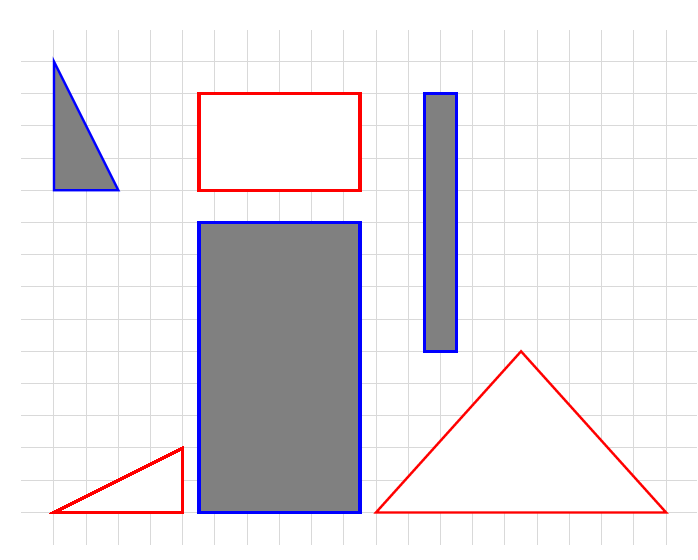
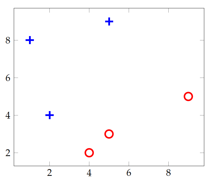
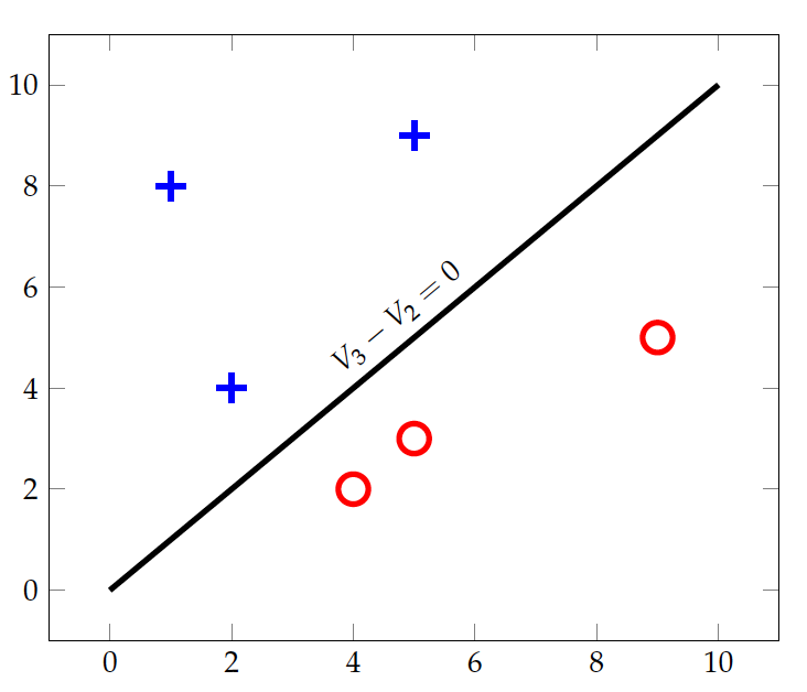
We shall continue to use a simple data set we encountered earlier, namely the instances of shapes on the concept of standing vs. lying. Suppose we have identified width and height as relevant attributes to the concept and Table tab:bin:shapes shows the data:
| Width | Height | Standing? | |
|---|---|---|---|
| 4 | 2 | No | |
| 5 | 9 | Yes | |
| 9 | 5 | No | |
| 2 | 4 | Yes | |
| 1 | 8 | Yes | |
| 5 | 3 | No |
Shapes data
If the shape instances here can serve as training data, how can an algorithm identify the relation between width and height as a predictor for the concept of standing?
Given this simple problem – simple to the human eye – it may be tempting to hardcode a selection structure such as height>width? into an algorithm and make predictions without the training data. This, however, defeats the purpose of data-driven machine learning. While we can easily identify the classification rule with this small data set, it is impossible to do so with massive data and more complex relations.
We should instead design a general strategy by which related rules and relations can be captured from training data and then used in predictions. What potential strategies can we propose? Let’s look at a few proposals.
The easiest approach to learning is not to learn at all, or simply memorize all given materials without trying to understand them. We can refer to this as lazy learning, which is similar to what some "lazy" students may do in reality.
But in the real world, how does a student perform on a test (examination) if she has not understood anything at all? The solution is to search, whether it is searching one’s memory or materials and notes. Without understanding, one will try to find notes and sections most closely related to a test question and develop an answer based on the search result.
Likewise, in machine learning, a lazy learning method
- does not build any model at all but simply remembers (stores) training instances.
To predict on a test instance, the method
- searches its memory (training data), finds the most closely related instances to the test,
- and predicts the answer based on related instances it has found.
- Nearest neighbors: closely related instances
- kNN: predicts based on k closet training instances
We normally refer to the most closely related instances as the nearest neighbors. A classic lazy learning algorithm is the k nearest neighbors (kNN) approach, which makes predictions based on k closest training instances.
But how does the algorithm find out which ones are the nearest? It needs a function to measure the closeness or distance between two instances. An example of such a distance function is the Euclidean distance, which the length a straight line connecting the endpoints of two instances u and v in dimensional space.
Euclidean distance: \begin{eqnarray} D(u,v) & = & \sqrt{\sum_{i=1}^{m} (u_i - v_i)^2}\end{eqnarray}
where m is the number of dimensions (features) to represent each data instance. Figure fig:bin:ed shows the shapes data on two dimensions, i.e. width and height. Suppose a new instance at (4,7), i.e. width=4 and height=7, is to be tested. The dashed lines are the euclidean distances from the test instance to the training instances.
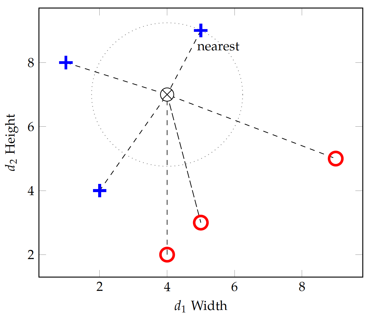
If we set k=1 for the kNN algorithm, we will use only 1 nearest neighbor in prediction. The instance at (5,9), which belongs to the standing class, has a distance from the test instance:
This turns out to be the nearest in terms of Euclidean distance and the test instance will be predicted standing (positive) as well. If we change k=3, the 3 nearest neighbors will all be positive (+) instances and the prediction for the above test instance will remain positive.
For a different test instance, the k nearest neighbors might have conflicting answers. For binary classification, one strategy is to pick an odd number for k and let the nearest neighbors vote for the final prediction.
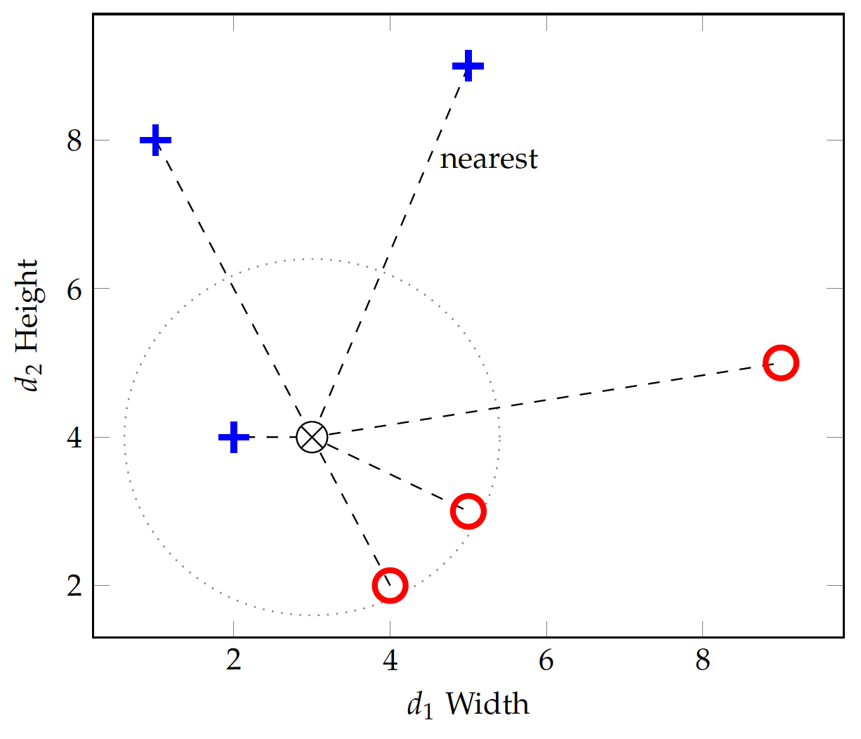
Figure fig:bin:ed2 shows another test instance at (3,4). With k=3, it turns out that the three nearest neighbors include 1 positive and 2 negatives. Using a majority vote strategy, the test instance will be mistakenly classified into the negative (lying) class.
Two observations on the misclassification. First, the selection of k does have an impact on the classification result. This is especially true when training instances are sparse. With k=1, the method relies on one single instance for each test and is hardly robust. A larger k can reduce the likelihood of predicting with atypical neighbors but it introduces noise, e.g. instances from across the class boundary as illustrated in Figure fig:bin:ed2. Finding the optimal k may require experimentation with data.
Second, more important, a lazy learner such as kNN does not have a general function (model) to represent a concept of learning. It purely relies on individual training instances for predictions and has no generalizability. Its success or failure depends on where the test instance hit and how training data distribute around it. This is analogous to a lazy student who memorizes everything without understanding – she will not be able to answer a question for which no similar examples have been provided in the materials.
Euclidean distance is a special case of a category of distance metrics known as the Minkowski distance, which is defined as:
where $p \ge 1$ and m is the number of dimensions. When $p=2$, this is the Euclidean distance.
When p=1, it becomes the Manhattan distance:
\begin{eqnarray} MD_1(u, v) & = & \sum_{i=1}^{m} |u_i - v_i|\end{eqnarray}which is similar to counting the number of blocks in a city grid.
Another metric is similar to (but not exactly) Minkowski distance with p=0:
\begin{eqnarray} MD_0(u, v) & = & \sum_{i=1}^{m} (u_i - v_i)^0 \\ & = & \sum_{u_i \ne v_i} 1\end{eqnarray}which counts the number of dimensions where there is a difference and is often referred to as edit distance. This is equivalent to treating every dimension as a binary variable and the overall distance is the amount of change in the bits.
As we observed, a lazy learner such as the k Nearest Neighbors (kNN) does not actually learn and build a model (function) that can be generalized. Although kNN has decent performances in many applications, it suffers in domains where, for example, test data appear on a different scale from that of training data.
If we assume the classes can be separated by a function (model) with certain parameters, then building the model requires identification of those parameters from training data. Surely there are way too many different functional forms one can choose the model from. We start with the simplest, a linear function.
| x ($v_1$) | y ($v_2$) | class |
|---|---|---|
| 4 | 2 | No |
| 5 | 9 | Yes |
| 9 | 5 | No |
| . | . | .. |
With the shapes data in Figure fig:bin:ed, there are two variables width (v_1 for the x axis) and height (v_2 for y axis). y as a linear function of x can be written as f(x) = a + b x or a + b x - y = 0, with two parameters a and b for two variables.
The specific model we can identify for the data here is:
And the linear equation that separates the two classes is: $$ x - y = 0 $$
Or $$ v_1 - v_2 = 0 $$
That is: $$ 0 + 1 \times v_1 - 1 \times v_2 = 0$$
OR: $$ w_0 + w_1 v_1 + w_2 v_2 = 0$$
where the $w$ parameters can be estimated. For the model here, $w_0 = 0$, $w_1 = 1$, and $w_2 = -1$.
When there are more variables (dimensions), the function can be extended to:
That is: \begin{eqnarray} w_0 + \sum_{i=1}^{m} w_i v_i & = & 0 \label{eq:bin:lin}\end{eqnarray}
where m is the number of variables (dimensions).
With m=2 for the shapes data, how do we estimate the parameters w_0, w_1, and w_2 in Equation eq:bin:lin2 to linearly separate the two classes standing vs. lying? Note that a linear equation in a 2-dimensional space is a straight line. It is a plane (flat surface)) in a 3-dimensional space and a hyperplane in a higher-dimensional space.1 We will discuss several approaches of the linear model.
We start with finding the centroid for instances in each class. A centroid is the center of the mass for a group of objects and can be computed as the average of values on each dimension.
The $j^{th}$ dimension of the centroid for class c is computed by:
\begin{eqnarray} \mu_{j}(c) & = & \frac{\sum_{i=1}^{n_c} v_{ij}}{n_c}\end{eqnarray}where $v_{ij}$ is the value of the $j^{th}$ dimension of the $i^{th}$ instance in class c.
Following this equation, the centroids for the positive (standing) and negative (lying) classes can be obtained:
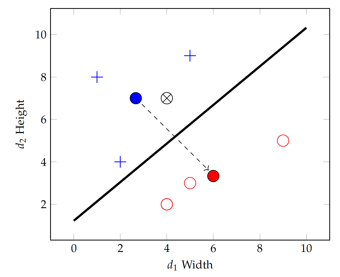
Figure fig:bin:lin_cent shows the two centroids and a dashed line with an arrowhead connecting them. The arrow represents a vector in the direction \vec{\mu} = (6-\frac{8}{3}, \frac{10}{3} - 7) = (\frac{10}{3}, - \frac{11}{3}), whereas the middle of the dashed line is \bar{\mu} = (\frac{13}{3}, \frac{31}{6}).
Now if we can find a linear equation, i.e. another straight line, that: 1) passes through the middle of the dashed line (equal to each centroid), and 2) is perpendicular to the dashed line, then any point on the linear equation (line) should have an equal distance from both centroid. In this case, the line can serve as the boundary between the two classes.
Now, identifying the linear equation turns out to be very straightforward.
The middle point of $\mu(\oplus)$ and $\mu(\ominus)$ is: $$ \bar{\mu} = (\frac{13}{3}, - \frac{31}{6}) $$
For any point $(v_1, v_2)$, it can be seen as a vector originated from the midle point:
\begin{eqnarray} \vec{v} & = & (v_1 - \frac{13}{3}, v_2 - \frac{31}{6})\end{eqnarray}For the vector to be perpendicular to the dashed vector $\vec{\mu}$, their dot product should be 0. That is:
which is:
or:
Comparing this to Equation eq:bin:lin2, we have identified the parameters w_0=-1, w_1=-\frac{20}{27}, and w_2=\frac{22}{27} for the linear classification function. This is the solid straight line separating the two classes (centroids) in Figure fig:bin:lin_cent.
With the identified linear function $f(v) = 1 + \frac{20}{27} v_1 - \frac{22}{27} v_2$, one can plug in values of a test instance and make a prediction. If the result is positive, it will predict positive (standing); otherwise, it will predict negative (lying). For example, given a test instance at (4,7) ($\otimes$ on Figure fig:bin:lin_cent), we can put the values in the linear function and get:
The final result is positive – the same positivity with the positive class centroid – and hence the test instance \otimes will be classified into the standing class.
Theoretically, we understand that the concept of standing is on the relation of height - width >0 or, in terms of the linear function, 0 - v_1 + v_2 > 0. The identified equation is a rough approximation of this theoretical function. The model assumption about a linear separation holds true in this example. But how precise we can establish the exact linear function greatly depends on the training data. The data distribution influences the identification of related parameters.
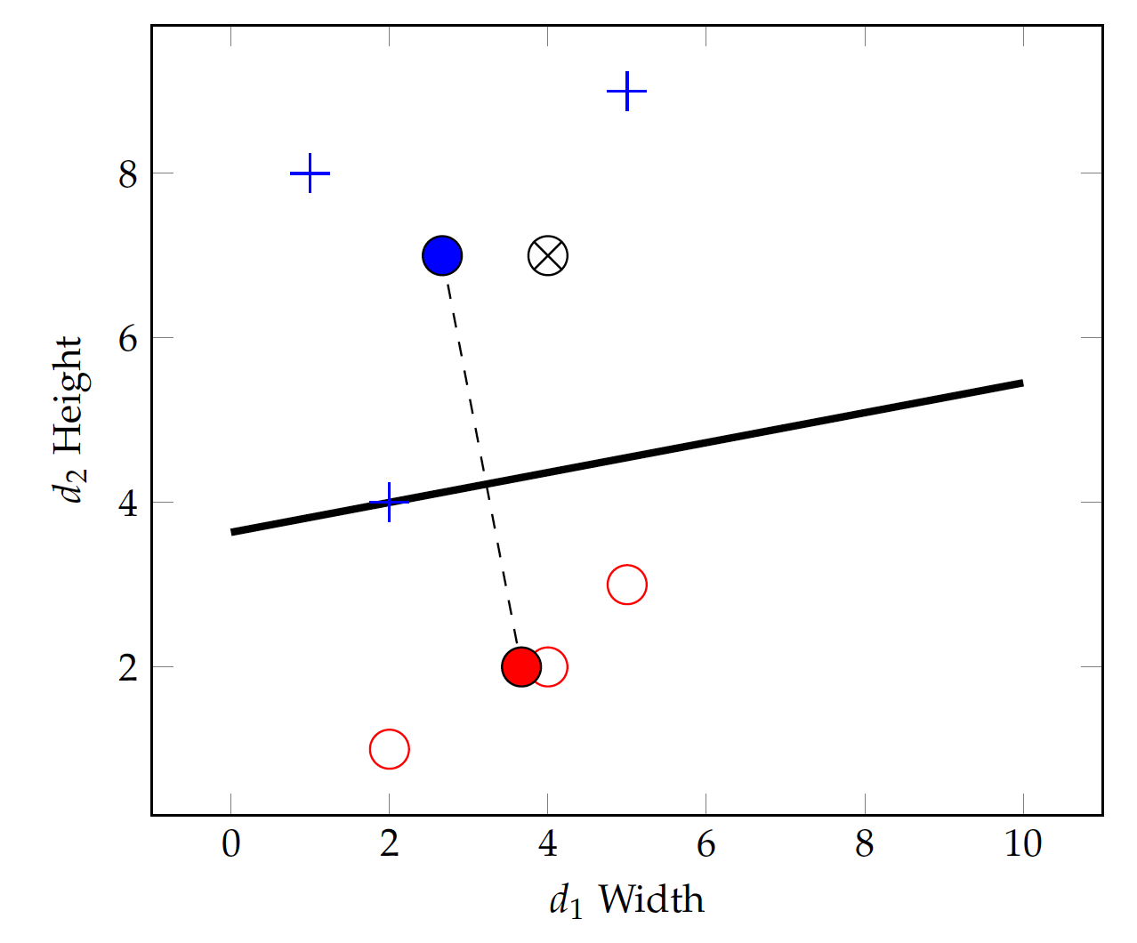
In particular, the centroid approach is greatly impacted by the density of the training set and where most data instances are. For example, having more data instances with smaller width and height in the negative class change its centroid, which will, in turn, lead to a very different linear function, illustrated in Figure fig:bin:lin_cent2 (compare to Figure fig:bin:lin_cent).
The centroid-based approach to linear classification is greatly influenced by all data points in the training set and how they are distributed. The basic assumption underlying the above modeling is that the two classes are of the same size roughly and the "border" lies halfway between their centers. This is often untrue and its performance suffers.