
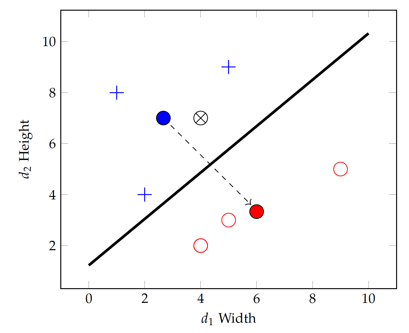
Following this equation, the centroids for the positive (standing) and negative (lying) classes can be obtained:
Rather, it is much more relevant to find out where cities, landmarks, and populations are on the border.
For U.S. and Canada, cities such as Seattle vs. Detroit vs. Vancouver, Detroit vs. Toronto help define their border.
For classification, it matters not where the centroids are but where the borderline data are. The Support Vector Machines, or SVM, is a method focused on the border populations and draws the "border" based on the so-called support vectors, data points that are located on the boundary and together form the border.
We start by connecting a number of data points within the same class to construct a linear function, i.e. a line on a 2-dimensional space, a plane for 3 dimensions, and a hyperplane for higher dimensions. On the 2-dimensional shapes data, this means using any two points in each class to form a straight line that, when used as the linear classification function, satisfies two conditions.
Candidate support vectors, data pairs in each class to form lines where:
- all data points in the same class fall on one side of the linear function, and
- most if not all data points of the other class reside on the other side of the line.
In other words, if a line is drawn in the positive (standing class), then 1) data in it will test all positive (or all negative), and 2) data in the other class will test the opposite, negative (or conversely positive).
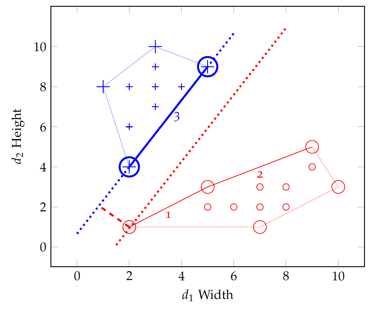
Figure fig:bin:svm illustrates the idea with the shapes data. 2 Pairwise lines drawn in the figure all satisfy the 1^{st} condition and collectively form a convex hull for each class. However, not all lines meet the 2^{nd} condition. In fact, only the lines marked 1, 2, and 3 meet both conditions. They are candidate support vectors.
For each of the three candidate lines, we can draw a line perpendicular to it from any point in the other class. From this process, we can find out the margin between that candidate support vector line and the other class (convex hull), which is where the boundary can be defined. For example, in Figure fig:bin:svm, the two dotted lines show the margin between line #3 and the negative class.
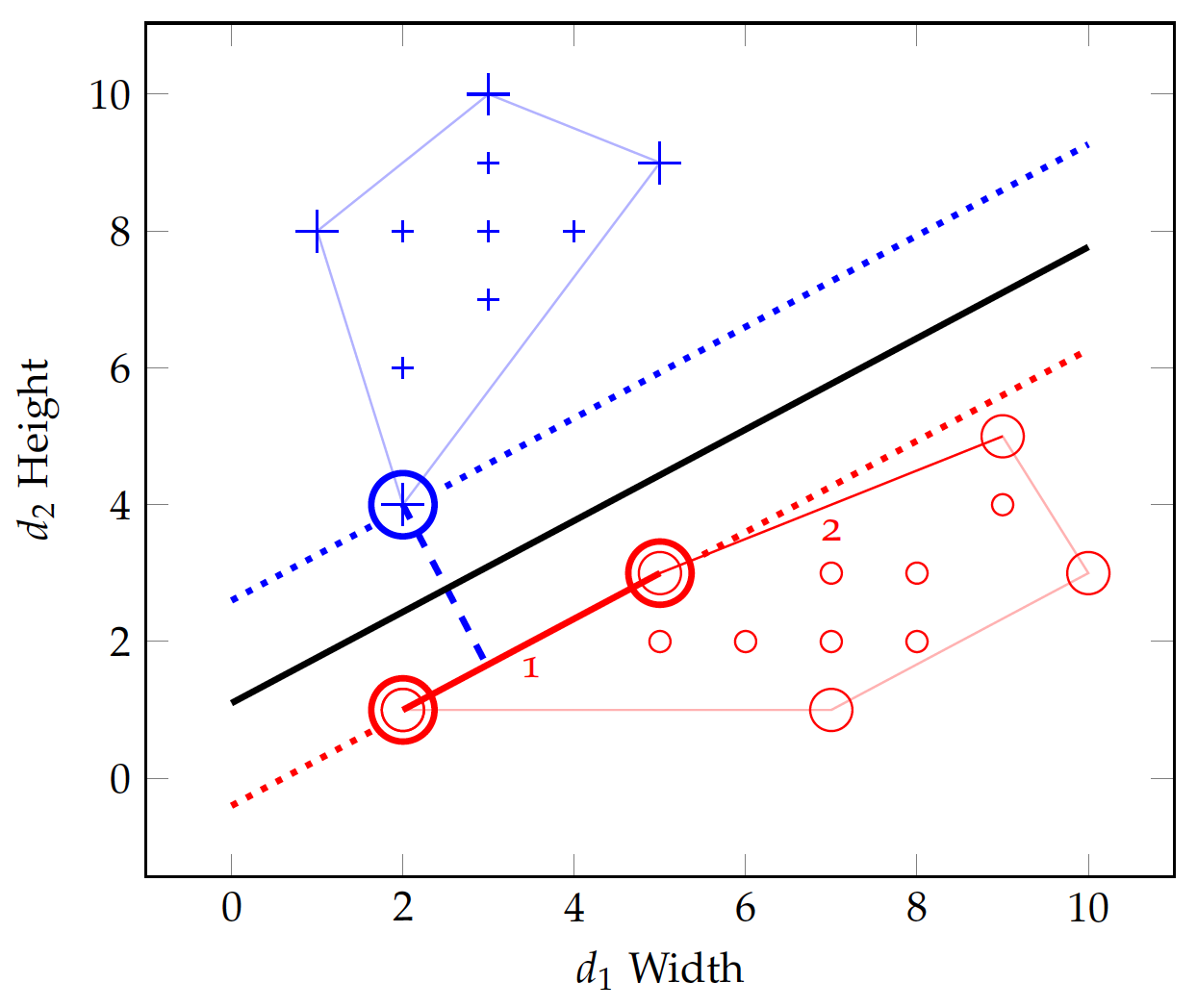
Yet a greater margin – in fact the greatest margin of all – can be found between line #1 and point (2,4) in the positive class, as the two dotted lines in Figure fig:bin:svm2 show. The greatest margin will be chosen as the decision boundary, which is defined by a few data points known as the support vectors. As shown as circled data points in Figure fig:bin:svm2, support vectors are those that determine the maximum margin between the two convex hulls of the two classes.
With this, it is now easy to identify the linear equation in the margin to separate the two classes. In Figure fig:bin:svm2, for example, the solid line at v_2 = 1.1 + 0.667 v_1 can be used as the linear classifier. One can certainly use the linear functions on the support vectors for classification as well, e.g. to predict one class vs. another if a test instance is within the support vector boundary or to estimate a probability if it is on the margin.
Note that with the shapes data example, we only have to deal with two dimensions and any linear equation is a straight line. With a higher dimensionality, the process remains the same mathematically but a linear function becomes a plane or hyperplane. On three dimensions, for example, three data points should be connected to construct a linear equation (plane) to identify the convex hulls and support vectors. Chapter has details on the mathematics for SVM.
A linear function $f(v)=w_0 + w_1 v_1 + w_2 v_2$ can be visualized as a perceptron:

where the node at $\sum$ computes the weighted sum of input variables. Obviously, this can be extended to include any number of variables m for which $f(v)=\sum_{i=1}^{m} w_i v_i$.
A perceptron is a simple, one-layer neural network – besides the input variables, there is only one layer of nodes (only one \sum node) in the model, as shown in Figure fig:bin:perceptron. The final output of the perceptron is binary 0 or 1 by using a step function, which simply converts values higher than a threshold to 1 and those lower to 0.
For example, one can use 0 as the threshold for a
step function f(s):
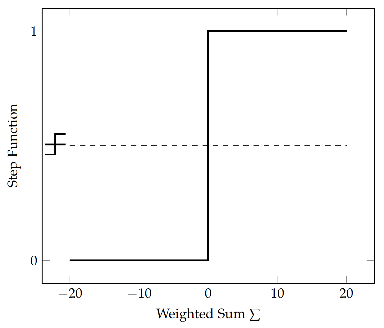
which is visualized in Figure fig:bin:step.
Before training, the weights are unknown and should be initialized with certain values, e.g. all 0. For each training instance, its values v_1 and v_2 will be fed into the input layer and multiplied with their weights w_1 and w_2 respectively.
Note that in Figure fig:bin:perceptron, the input with weight w_0 is always 1 for every training instance. This is referred to as the bias, which adds the constant w_0 to the linear function. Once every input is multiplied by its weight, the output computes the sum of the weighted values.
For the shapes data, we can decide that the model will predict positive (standing) if the output is greater than 0; negative (lying) if otherwise. During training, if a correct prediction is made, the model will have no need to adjust its weights (for now) and will simply move to the next training instance.
If a misclassification occurs, however, the model will have to adjust its weights so it can potentially make more correct predictions in the future. When the model predicts negative on an actual positive instance, the weights should be adjusted so the overall output (sum) will move toward the positive side; and vice versa.
For a positive (+) case predicted to be negative (-):
| v1 Width | v2 Height | Standing? |
|---|---|---|
| 5 | 9 | Yes |
Adjust after the false negative case:
\begin{eqnarray} w'_0 & \gets & w_0 + 1 \\ w'_1 & \gets & w_1 + v_1 \\ w'_2 & \gets & w_2 + v_2\end{eqnarray}For example, for a specific shape instance with v_1 (width) and v_2 (height) values, which is (1, v_1, v_2) with the bias input included. Suppose v_2>v_1 and this instance actually belongs to the positive (standing) class. Now if the model finds out w_0 + w_1 v_1 + w_2 v_2 < 0 and predicts negative (lying). We will add the input values to their current weights:
where w' is the updated weight. Because v_2>v_1, the weight for height w_2 will increase more than the weight for width w_1.
Conversely, for a training instance with v_1>v_2 that actually belongs to the negative (lying) class, if it is misclassified as positive, then the current weights will be reduced by the input values:
For a negative (-) case predicted to be positive (+):
| v1 Width | v2 Height | Standing? |
|---|---|---|
| 4 | 2 | No |
Adjust after the false positive: \begin{eqnarray} w'_0 & \gets & w_0 - 1 \\ w'_1 & \gets & w_1 - v_1 \\ w'_2 & \gets & w_2 - v_2\end{eqnarray}
Now that v_1>v_2, the weight for width w_1 will be reduced more than w_2. The training continues for a number of iterations or until the weights stabilize. With more training instances and misclassifications, the weights will be adjusted further, leading to relatively a greater (positive) value of w_2 and a smaller (negative) value of w_1.
Theoretically, we know that the classification function for standing vs. lying should be in the form of f(v) = 0 - v_1 + v_2, with w_1 and w_2 having opposite signs. Overall, the adjustment of weights discussed above is moving in the correct direction. As for the bias, it will simply be adjusted back and forth with positive and negative misclassifications. For the shapes data, w_0 will be more or less canceled out and its absolute value will become much smaller than those of w_1 and w_2.
The perception model is learning by mistakes, as it updates the weights only when there is misclassification. For classes that are linearly separable, the updating strategy is guaranteed to converge on a set of weights.